FIFI-LS Redux User’s Manual

Introduction

The SI Pipeline Users Manual (OP10) is intended for use by both SOFIA Science Center staff during routine data processing and analysis, and also as a reference for General Investigators (GIs) and archive users to understand how the data in which they are interested was processed. This manual is intended to provide all the needed information to execute the SI Level 2/3/4 Pipeline, and assess the data quality of the resulting products. It will also provide a description of the algorithms used by the pipeline and both the final and intermediate data products.

A description of the current pipeline capabilities, testing results, known issues, and installation procedures are documented in the SI Pipeline Software Version Description Document (SVDD, SW06, DOCREF). The overall Verification and Validation (V&V) approach can be found in the Data Processing System V&V Plan (SV01-2232). Both documents can be obtained from the SOFIA document library in Windchill.

This manual applies to FIFI-LS Redux version 2.7.0.

SI Observing Modes Supported

FIFI-LS Instrument Information

FIFI-LS has two separate and independent grating spectrometers with common fore-optics feeding two large Ge:Ga detector arrays (16 x 25 pixels each). The wavelength ranges of the two spectral channels are 42 - 110 microns and 110 - 210 microns, referred to as the BLUE and RED channels, respectively.

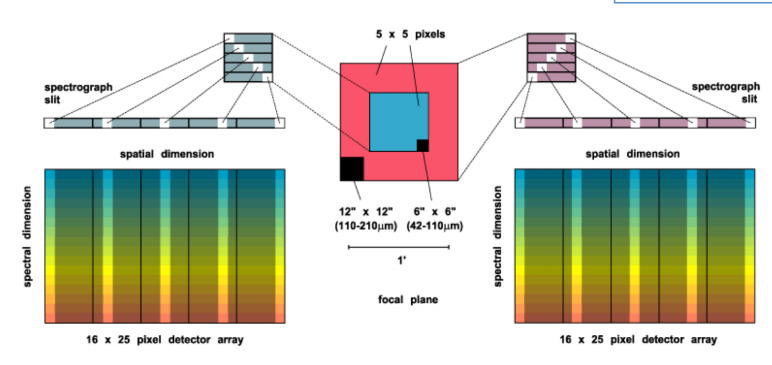
Fig. 19 The integral field unit for each channel

Multiplexing takes place both spectrally and spatially. An image slicer redistributes 5 x 5 pixel spatial fields-of-view (approximately diffraction-limited in each wave band) along the 1 x 25 pixel entrance slits of the spectrometers. Anamorphic collimator mirrors help keep the spectrometer compact in the cross-dispersion direction. The spectrally dispersed images of the slits are anamorphically projected onto the detector arrays, to independently match spectral and spatial resolution to detector size, thus enabling instantaneous coverage over a velocity range of ~ 1500 to 3000 km/s around selected FIR spectral lines, for each of the 25 spatial pixels (“spaxels”).

The detectors are read out with integrating amplifiers: at each pixel a current proportional to the incident flux charges a capacitor. The resulting voltage is sampled at about 256Hz. After a certain number of read-outs (the ramp length), the capacitors are reset to prevent saturation. Thus, the data consist of linearly rising ramps for which the slope is proportional to the flux. See Fig. 20 for an illustration of the read-out sequence.

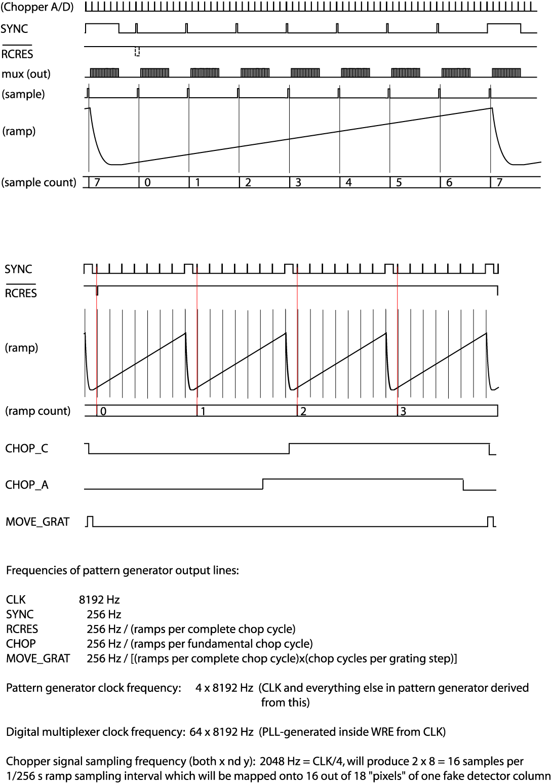
Fig. 20 FIFI-LS readout sequence

FIFI-LS Observing Modes

Symmetric chop mode, also known as nod-match-chop mode, is the most common observing mode. In this mode, the telescope chops symmetrically to its optical axis, with a matched telescope nod to remove background. A typical observation sequence will cycle through the A nod position and the B nod position in an ABBA pattern.

Most observations will be taken using symmetric chop mode. However, if the object is very bright, the efficiency is improved by observing in an asymmetric chopping mode. This mode typically consists of two map positions and one off-position per nod-cycle (an AAB pattern, where the B position contains only empty sky). Asymmetric chopping may also be used if an object’s size requires a larger chop throw than is possible with symmetric chopping.

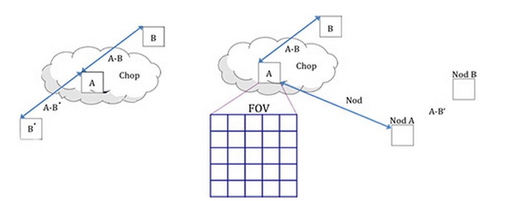
Fig. 21 The geometry of chopping and nodding in the symmetric chop mode (left) and the asymmetric mode (right).

Occasionally, for very bright targets, it may be advantageous to take data with no chopping at all. This mode, called total power mode, may be taken with either symmetric or asymmetric nodding for sky subtraction, or with no nods at all.

For extended targets, total power observations may also be taken in on-the-fly (OTF) scanning mode. In this mode, the telescope is continuously scanned across the target, at a speed calculated for minimal smearing within a single ramp. Each ramp is then treated as if it were a separate observation (A nod), with its own position coordinates. The sky position (B nod) may be observed separately, before or after the OTF scan, similar to the asymmetric nodding method. The sky position is not scanned.

At each chop and nod position (on- and off-position), it is common to step the grating through a number of positions before each telescope move. These additional grating scans effectively increase the wavelength coverage of the observation. Note, however, that grating scans are not used with the OTF mode, due to the continuous telescope motion.

Algorithm Description

Overview of Data Reduction Steps

This section will describe, in general terms, the major algorithms used to reduce a FIFI-LS observation. See Fig. 22 for a flow chart showing how these algorithms fit together.

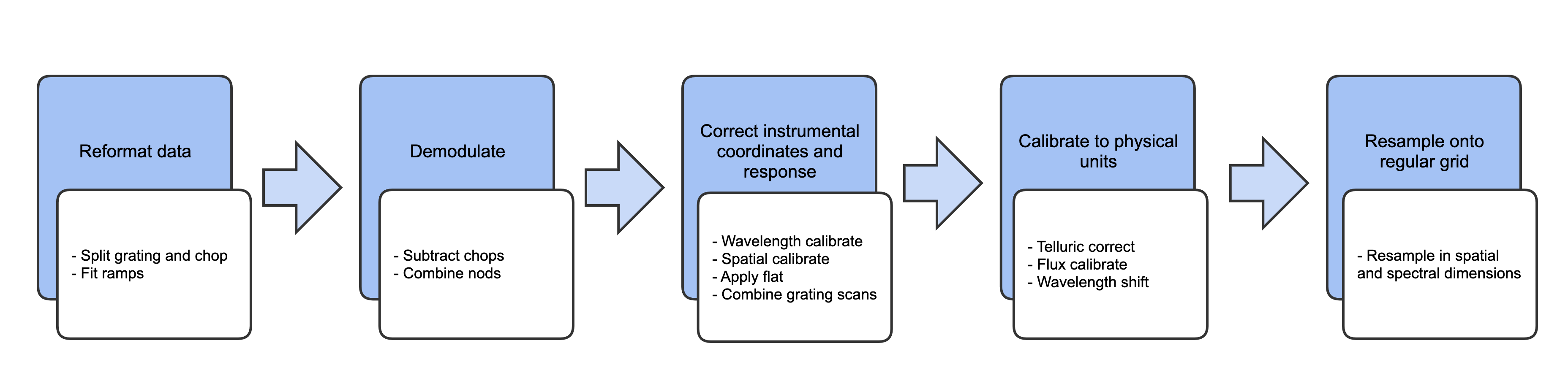
Fig. 22 Processing steps for FIFI-LS data. The blue box describes an overview of the steps and the white box contains the actual steps carried out.

Reduction Algorithms

The following subsections detail each of the data reduction pipeline steps outlined in the flowchart above.

Split Grating and Chop

A single FIFI-LS raw FITS file contains the data from both chop positions (on and off) for each grating step used in a single nod position. FIFI-LS records its grating positions in “inductosyn” units. These are long integer values that are used to convert the data to a micron scale in the wavelength calibrate step.

The raw FIFI-LS data consist of a header (metadata describing the observation) and a table of voltage readings from the detector pixels. Each data section contains one frame, i.e. simultaneous readouts of all detector pixels and grating values.

The data header is sent before each frame. The following 8 unsigned 16-bit words contain the header information.

• Word 0: The word #8000 marks the start of the header.

• Word 1: The low word of the 32-bit frame counter.

• Word 2: The high word of the 32-bit frame counter.

• Word 3: The flag word. Bit 0 is the chopper signal. Bit 1 is the detector (0=red, 1=blue). Unused bits are fixed to 1 to recognize this flag word.

• Word 4: The sample count as defined in the timing diagrams (see Fig. 20). This count gets advanced at every sync pulse and reset at every long sync pulse.

• Word 5: The ramp count as defined in the timing diagrams. This counter gets advanced with a long sync pulse and reset by RCRES.

• Word 6: The scan index

• Word 7: A spare word (for now used as “end of header”: #7FFF).

Only columns 3, 4, and 5 are used in the split grating/chop step. The following shows example header values for a raw RED FIFI-LS file:

columns:
  0     1     2     3     4     5     6     7
-----------------------------------------------
32768 28160  15     1     0     0    89   32767
32768 28161  15     1     1     0    89   32767
32768 28162  15     1     2     0    89   32767
32768 28163  15     1     3     0    89   32767
32768 28164  15     1     4     0    89   32767
32768 28165  15     1     5     0    89   32767
32768 28166  15     1     6     0    89   32767
32768 28167  15     1     7     0    89   32767
32768 28168  15     1     8     0    89   32767
32768 28169  15     1     9     0    89   32767
32768 28170  15     1    10     0    89   32767
32768 28171  15     1    11     0    89   32767
...

Column 3 is all ones, indicating that the data is for the RED channel, column 4 counts the readouts from 0 to 31, and column 5 indicates the ramp number.

Where each chop and grating position starts and stops in the raw data table is determined using the header keywords RAMPLN_[B,R], C_CYC_[B,R], C_CHOPLN, G_PSUP_[B,R], G_PSDN_[B,R] keywords. A RED data example is as follows:

RAMPLN_R= 32 / number of readouts per red ramp
C_CHOPLN= 64 / number of readouts per chop position
G_PSUP_R= 5  / number of grating position up in one cycle
G_PSDN_R= 0  / number of grating position down in one cycle

Here, C_CHOPLN / RAMPLN_R is 64 / 32 = 2; therefore, there are 2 ramps per chop.

Each chop switch index is determined using the 5^th column in the header. It is chop 0 if the value is odd and chop 1 if the value is even. Grating scan information determines how that chop phase is split up into separate extensions using the following formula:

\[binsize = (nreadout * ramplength) / (nstep * choplength)\]

where nreadout is the total number of readouts (frames) in the file, ramplength is determined by the appropriate RAMPLN keyword, nstep is the number of grating steps (G_PSDN + G_PSUP), and choplength is the number of readouts per chop position (C_CHOPLN).

The binary data section is comprised of 468 signed 16-bit words: one each for 25 spaxels, plus one control value, times 18 spectral channels (“spexels”). The spaxels are read out one spectral channel at a time. Spectral channel zero of all 25 pixels are read out, and then a grating value (analog readout from the grating mechanism) is recorded; then the next channel of all the pixels is read out, and then the next grating value, and so on, through all the spectral channels. The grating values may be during pipeline processing to discard samples with inconsistent grating positions, but are then discarded for further processing. Of the 18 spectral channels, channel 0 is the CRE resistor row and row 17 is the empty CRE row (“dummy channel”). The empty row may be used during processing, to help remove correlated noise from a spaxel. These two channels are then discarded; the other 16 channels are considered valid spexels.

The first step in the data reduction pipeline is to split out the data from each grating scan position into separate FITS image extensions, and to save all grating positions from a single chop position into a common file. For example, if there are five grating scans per chop, and two chop positions, then a single one-extension input raw FITS file will be reorganized into two files (chop 0 and chop 1) with 5 extensions each. For total power mode, there is only one chop position, so there will be one output file, with one extension for each grating step. Each extension in the output FITS files contains the data array corresponding to the grating position recorded in its header (keyword INDPOS). Hereafter, in the pipeline, until the Combine Grating Scans step, each grating scan is handled separately.

For OTF mode data, an additional binary table is attached to the FITS file, recording the telescope position at each readout sample. These positions are calculated from the telescope speed keywords in the FITS header (OBSLAMV and OBSBETV, for RA and Dec speeds in arcsec/s, respectively). Readouts taken before and after the telescope scanning motion are also identified using the OTFSTART and TRK_DRTN header keywords. These readouts are flagged in the SCANPOS table for removal from consideration in later pipeline steps.

Fit Ramps

The flux measured in each spatial and spectral pixel is reconstructed from the readout frames by fitting a line to the voltage ramps. The slope of the line corresponds to the flux value.

Before fitting a line to a ramp, some likely bad frames are removed from the data. The grating values (in the 26^th spaxel position), the first ramp from each spaxel, the first 2-3 readouts per ramp, and the last readout per ramp are all removed before fitting.

Optionally, the flux in the first (empty) spectral pixel may be subtracted from all other spexels in its associated spaxel, as a correction for detector readout bias. The dummy channels in the first and last spectral pixels are then removed from the flux array; they are not propagated through the rest of the pipeline.

Additionally, the grating values in the spare spaxel may be used to identify ramps for which the grating deviated from the expected position. The grating values are averaged over a ramp, and compared to the expected value. If they do not fall within a threshold of the expected position, the ramp is flagged for rejection.

A ramp may be marked as saturated if it does not have its highest peak in the last readout of the ramp. If this occurs, the readout before the highest peak is removed before fitting, along with any readouts after it. This ensures that the slope is not contaminated by any non-linearity near the saturation point.

Typically, multiple ramps are taken at each chop position. After the slope of each ramp is derived, the slopes are combined with a robust weighted mean. This final averaged value is recorded as the flux for the pixel and the error on the mean is recorded as the error on the flux for that pixel. After this pipeline step, there is a flux value for each spatial and spectral pixel, recorded in a 25 x 16 data array in a separate FITS image extension for each grating scan. The error values are recorded in a separate 25 x 16 array, in another FITS image extension. The extensions are named with a suffix indicating the grating scan number. For example, for two grating scans, the output will have extensions FLUX_G0, STDDEV_G0, FLUX_G1, and STDDEV_G1.

For OTF data, each ramp represents a different sky position, so separate ramps are not averaged together, but are propagated through the pipeline as a data cube. The flux and error data arrays have dimension 25 x 16 x N_ramp, where N_ramp is the number of ramps for which the telescope motion was nominal. In the SCANPOS table attached to the FITS file, the telescope positions for each ramp are calculated from an average over the positions for the readouts in the ramp, and propagated forward for later use in spatial calibration.

Some pixels in the data array may be set to not-a-number (NaN). These are either known bad detector pixels, or pixels for which the ramp fits did not have sufficient signal-to-noise. These pixels will be ignored in all further reduction steps.

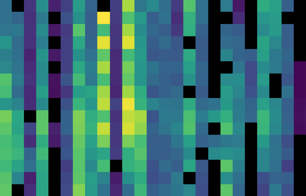
Fig. 23 The flux array from a single grating scan in the RED channel, at the chop 0 position in nod A after fitting ramps, flattened into a 25 x 16 array. The spectral dimension runs along the y-axis. The data was taken in symmetric chopping mode.

Subtract Chops

To remove instrument and sky background emission, the data from the two chop positions must be subtracted. For A nods in symmetric mode, chop 1 is subtracted from chop 0. For B nods in symmetric mode, chop 0 is subtracted from chop 1. All resulting source flux in the symmetric chop-subtracted data should therefore be positive, so that the nods are combined only by addition. In asymmetric mode, chop 1 is subtracted from chop 0 regardless of nod position.

This pipeline step produces one output file for each pair of input chop files. In total power mode, no chop subtraction is performed.

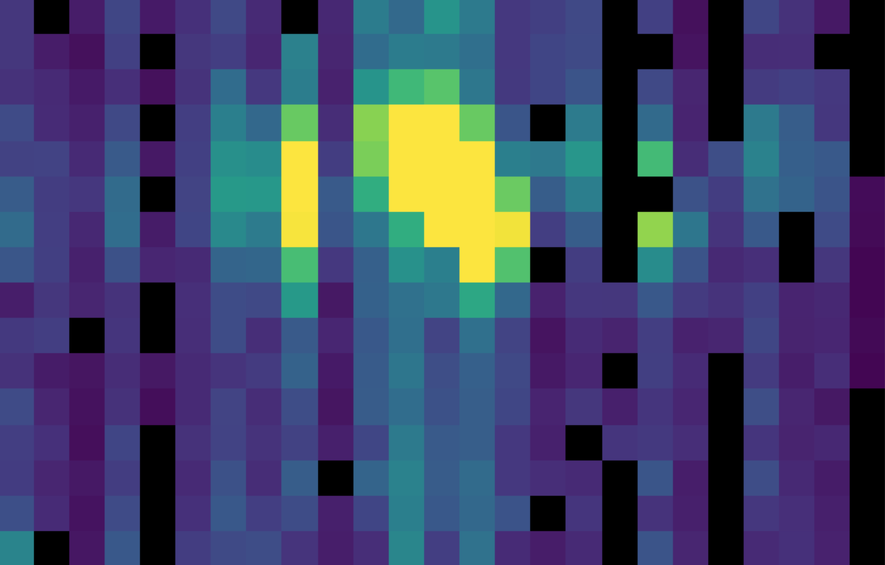
Fig. 24 The same flux array as in Fig. 23, with the corresponding chop 1 subtracted.

Combine Nods

After the chops are subtracted, the nods must be combined to remove residual background.

In symmetric chopping mode, the A nods are paired to adjacent B nods. In order to match a given A nod, a B nod must have been taken at the same dither position (FITS header keywords DLAM_MAP and DBET_MAP), and with the same grating position (INDPOS). The B nod meeting these conditions and taken nearest in time to the A nod (keyword DATE-OBS) is added to the A nod.

In asymmetric mode, a single B nod may be subtracted from multiple A nods. For example, in an AAB pattern the B nod is combined with each preceding A nod. The B nods in this mode need not have been taken at the same dither position as the A nods, but the grating position must still match. The matching B nod taken nearest in time is subtracted from each A nod.

Optionally, in asymmetric mode, the nearest B nods before and after the A nod may be combined before subtracting from the A nod, either by averaging them, or by linearly interpolating their values to the time of the A nod observation. In some cases, this may reduce background artifacts resulting from changes in the sky background between the A and B nod observations.

This pipeline step produces an output file for each input A nod file, containing the chop- and nod-combined flux and error values for each grating scan.

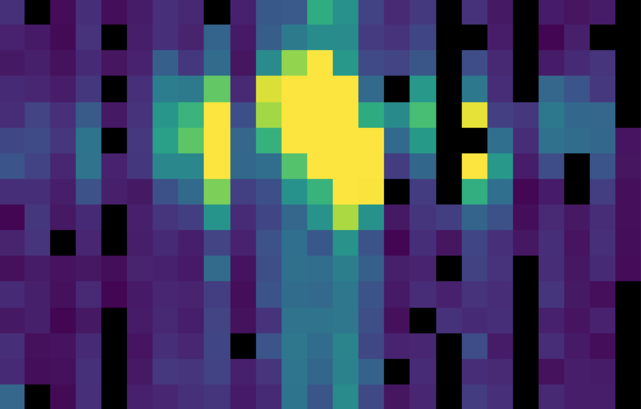
Fig. 25 The chop-subtracted symmetric mode nod A flux array, with the corresponding nod B added.

Wavelength Calibrate

The wavelength calibrate step calculates wavelength values in microns for each of the spectral pixels in each grating scan, based on the known grating position, a model of the optical geometry of the instrument, and measurements of the positions of known spectral lines. The optics within FIFI-LS tend to drift with time and therefore the FIFI-LS team updates the wavelength solution every year. The wavelength equation (below) is stored in a script, while all relevant constants are stored in a reference table, with an associated date of applicability.

The wavelength (\(\lambda\)) for the pixel at spatial position i and spectral position j is calculated from the equation:

\[\phi_{i} = \ 2\pi\ ISF\frac{ind + \text{ISOFF}_{i}}{2^{24}}\]

\[\delta_{j} = \ \left\lbrack j - 8.5 \right\rbrack*PS + sign\left\lbrack j - QOFF \right\rbrack*\left\lbrack j - QOFF \right\rbrack^{2}*QS\]

\[g_{i} = g_{0}*\cos\left( \frac{\text{SlitPos}_{i} - NP}{a} \right)\]

\[\lambda_{\text{ij}} = 1000\frac{g_{i}}{m}\left\lbrack \sin\left( \phi_{i} - \gamma \right) + \sin\left( \phi_{i} + \gamma + \delta_{j} \right) \right\rbrack\]

where:

\(ind\): the input inductosyn position

\(m\): the spectral order of the observation (1 or 2)

are inputs that depend on the observation settings, and

\(ISF\): inductosyn scaling factor

\(PS\): pixel scale, in radians

\(QOFF\): offset of quadratic pixel scale part from the “zero” pixel, in pixels

\(QS\): quadratic pixel scale correcting factor, in radians/pixel²

\(g_0\): grating constant

\(NP\): slit position offset

\(a\): slit position scale factor

\(\gamma\): offset from Littrow angle

are constants determined by the FIFI-LS team, and

\(ISOFF_i\): offset of the home position from grating normal in inductosyn units for the ith spaxel

\(SlitPos_i\): slit position of the ith spaxel

are values that depend on the spatial position of the pixel, also determined by the FIFI-LS team. The spaxels are ordered from 1 to 25 spatially as follows:

1	2	3	4	5
6	7	8	9	10
11	12	13	14	15
16	17	18	19	20
21	22	23	24	25

with corresponding slit position:

Slit position	Spaxel
1	21
2	22
3	23
4	24
5	25
6
7	16
8	17
9	18
10	19
11	20
12
13	11
14	12
15	13
16	14
17	15
18
19	6
20	7
21	8
22	9
23	10
24
25	1
26	2
27	3
28	4
29	5

Note that each spectral pixel has a different associated wavelength, but it also has a different effective spectral width. This width (\(d\lambda / dp\)) is calculated from the following equation:

\[d\lambda_{ij}/dp = 1000\frac{g_{i}}{m}\left\lbrack PS + 2*sign\left\lbrack j - QOFF \right\rbrack*\left( j - QOFF \right)*QS \right\rbrack\left\lbrack \cos\left( \phi_{i} + \gamma + \delta_{j} \right) \right\rbrack\]

where all variables and constants are defined above.

In order to propagate consistent values throughout the pipeline, all flux values are now divided by the spectral bin width in frequency units:

\[d\nu_{ij}/dp = (c / \lambda^2) (d\lambda_{ij}/dp)\]

The resulting flux density values (units \(ADU/sec/Hz\)) are propagated throughout the rest of the pipeline.

The wavelength values calculated by the pipeline for each pixel are stored in a new 25 x 16 array in an image extension for each grating scan (extension name LAMBDA_Gi for grating scan i).

Spatial Calibrate

The locations of the spaxels are not uniform across the detector, due to the optics not being perfectly aligned. See Fig. 26 for a plot of the average of the center of each spaxel location, as measured in the lab. This location is slightly different at each wavelength. These spaxel positions are determined by the FIFI-LS team and recorded in a look-up table.

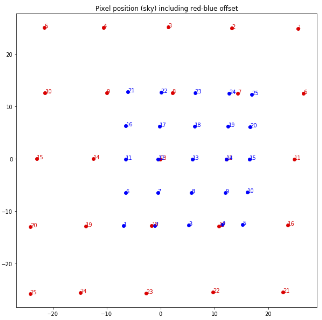
Fig. 26 Average fitted spaxel positions in arcsecond offsets from the center of the detector. The red dots indicate the positions for the RED channel; blue dots indicate the BLUE channel.

For a particular observation in standard chop-nod modes, the recorded dither offsets in arcseconds are used to calculate the x and y coordinates for the pixel in the ith spatial position and the jth spectral position using the following formulae:

\[x_{ij} = ps (xpos_{ij} + dx) + d\lambda cos(\theta) - d\beta sin(\theta)\]

\[y_{ij} = ps (ypos_{ij} + dy) + d\lambda sin(\theta) + d\beta cos(\theta)\]

where ps is the plate scale in arcseconds/mm (FITS header keyword PLATSCAL), \(d\lambda\) is the right ascension dither offset in arcseconds (keyword DLAM_MAP), \(d\beta\) is the declination dither offset in arcseconds (keyword DBET_MAP), \(\theta\) is the detector angle, \(xpos_{ij}\) and \(ypos_{ij}\) are the fitted spaxel positions in mm for pixel i,j, and dx and dy are the spatial offsets between the primary array (usually BLUE), used for telescope pointing, and the secondary array (usually RED). The dx and dy offsets also take into account a small offset between the instrument boresight and the telescope boresight, for both the primary and secondary arrays. By default, the coordinates are then rotated by the detector angle (minus 180 degrees), and the y-coordinates are inverted in order to set North up and East left in the final coordinate system:

\[x'_{ij} = -x_{ij} cos(\theta) + y_{ij} sin(\theta)\]

\[y'_{ij} = x_{ij} sin(\theta) + y_{ij} cos(\theta)\]

The pipeline stores these calculated x and y coordinates for each spaxel in two 25 element arrays for each grating scan (extensions XS_Gi and YS_Gi for grating scan i).

In addition, the pipeline uses the base position for the observation and the computed offsets to derive true sky coordinates for each spaxel, in RA (decimal hours) and Dec (decimal degrees). These positions are also stored in the output file in separate image extensions for each grating scan (RA_Gi and DEC_Gi for grating scan i), with array dimensions matching the corresponding XS and YS extensions.

For OTF data, the process is the same as described above, except that each ramp in the input data has its own DLAM_MAP and DBET_MAP value, recorded in the SCANPOS table, rather than in the primary FITS header. The output spatial coordinates match the number of spaxels and ramps in the flux data, which has dimensions 25 x 16 x N_ramp, such that the XS_Gi, YS_Gi, RA_Gi, and DEC_Gi, extensions have dimensions 25 x 1 x N_ramp.

Apply Flat

In order to correct for variations in response among the individual pixels, the FIFI-LS team has generated flat field data that correct for the differences in spatial and spectral response across the detector. There is a normalized spatial flat field for each of the RED and BLUE channels, in each of the dichroics, which specifies the correction for each spaxel. This correction may vary over time. There is also a set of spectral flat fields, for each channel, order, and dichroic, over the full wavelength range for the mode, which specifies the correction for each spexel.

In order to apply the flat fields to the data, the pipeline interpolates the appropriate spectral flat onto the wavelengths of the observation, for each spexel, then multiplies the value by the appropriate spatial flat. The flux is then divided by this correction value. The updated flux and associated error values are stored in the FLUX_Gi and STDDDEV_Gi extensions.

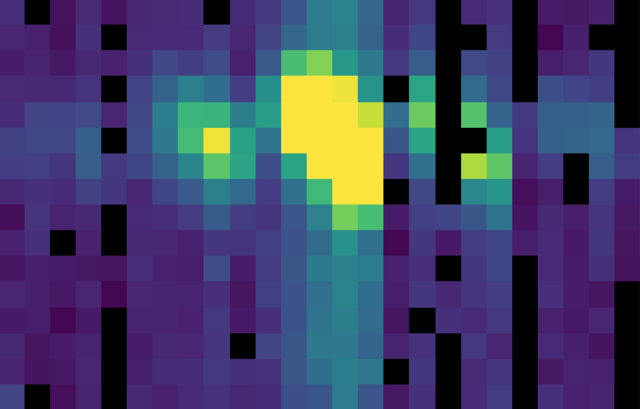
Fig. 27 The flat-corrected flux array.

Combine Grating Scans

Up until this point, all processing has been done on each grating scan separately. The pipeline now combines the data from all grating scans, in order to fill in the wavelength coverage of the observation.

Due to slight variations in the readout electronics, there may be additive offsets in the overall flux level recorded in each grating scan. To correct for this bias offset, the pipeline calculates the mean value of all pixels in the overlapping wavelength regions for each grating scan. This value, minus the mean over all scans, is subtracted from each grating scan, in order to set all extensions to a common bias level.

For standard chop/nod modes, the pipeline sorts the data from all grating scans by their associated wavelength values in microns, and stores the result in a single data array with dimensions 25 x (16 * N_scan), where N_scan is the total number of grating scans in the input file. Note that the wavelengths are still irregularly sampled at this point, due to the differing wavelength solutions for each grating scan and spatial pixel. All arrays in the output FITS file (FLUX, STDDEV, LAMBDA, XS, YS, RA, and DEC) now have dimensions 25 x (16 * N_scan).

For the OTF mode, only a single grating scan exists. The output FLUX, STDDEV, XS, YS, RA, and DEC arrays for this mode have dimensions 25 x 16 x N_ramp. Since the wavelength solution does not depend on the sky position, the LAMBDA array has dimensions 25 x 16.

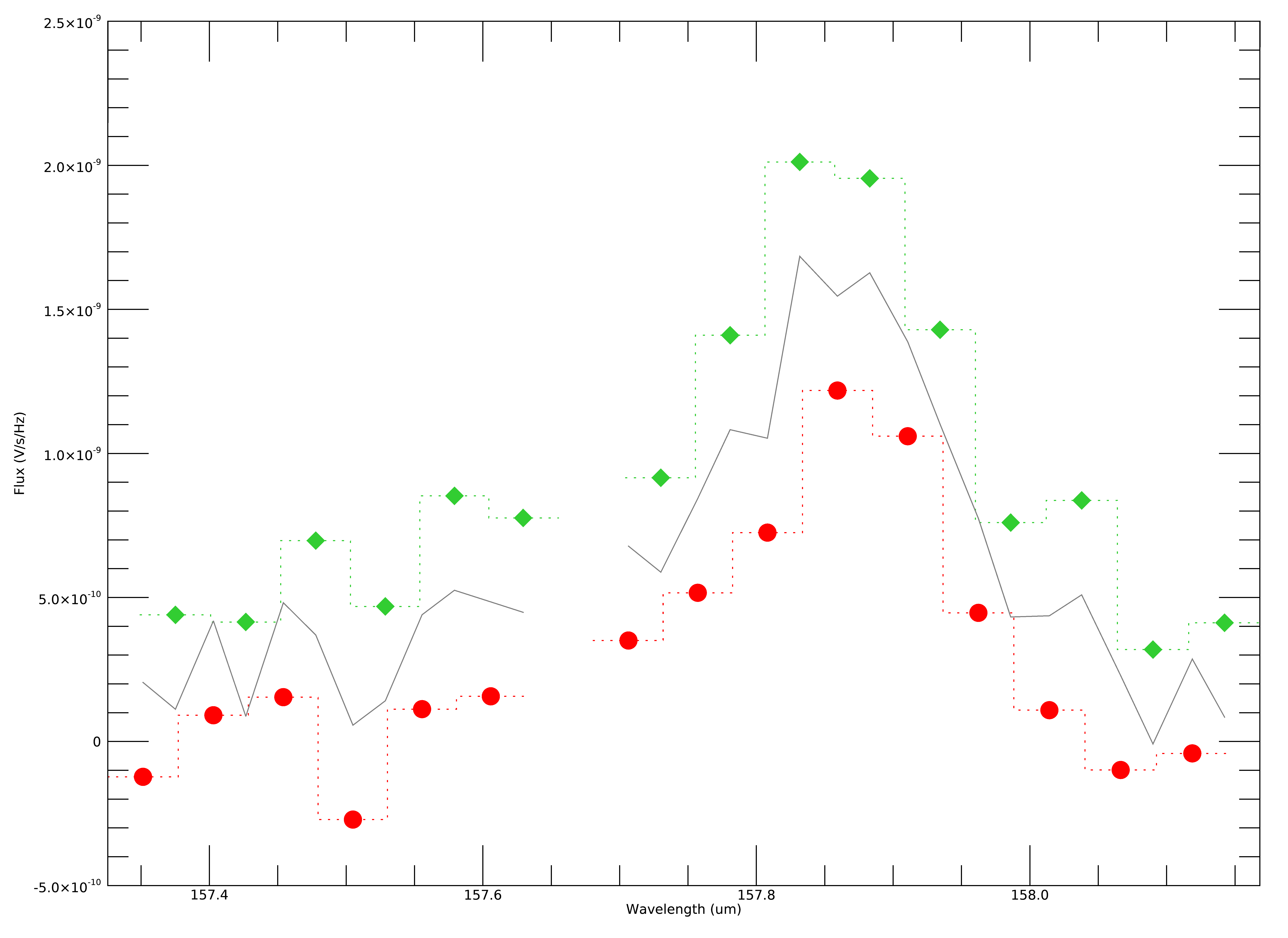
Fig. 28 Example spectral flux from the center spaxel for a single dither position. The red circles and green diamonds represents two different grating scans. The gray line indicates the combined flux array, after bias correction.

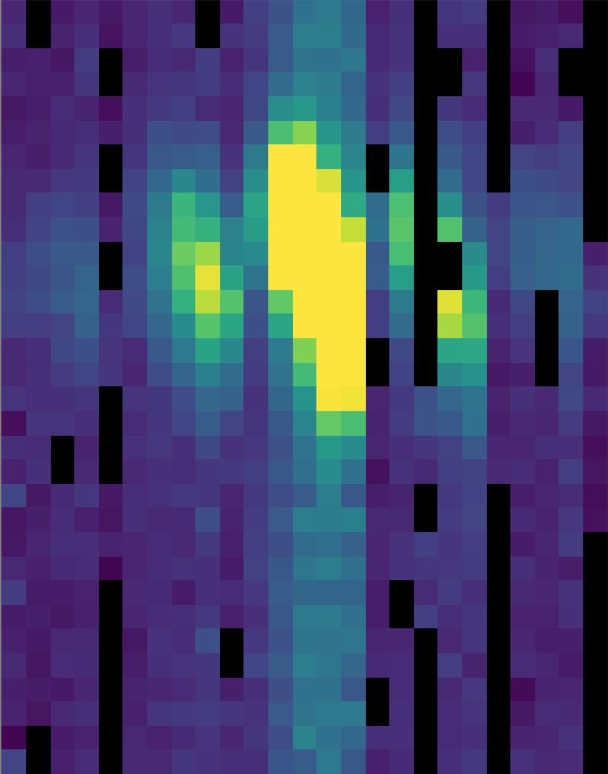
Fig. 29 The full 25 x 32 flux array, after combining two grating scans.

Telluric Correct

Telluric correction is the process of attempting to correct an observed spectrum for absorption by molecules in the earth’s atmosphere, in order to recover the intrinsic (“exo-atmospheric”) spectrum of the source. The atmospheric molecular components (primarily water, ozone, CO2) can produce both broad absorption features that are well resolved by FIFI-LS and narrow, unresolved features. The strongest absorption features are expected to be due to water. Because SOFIA travels quite large distances during even short observing legs, the water vapor content along the line of sight through the atmosphere can vary substantially on fairly short timescales during an observation. Therefore, observing a “telluric standard,” as is usually done for ground-based observations, will not necessarily provide an accurate absorption correction spectrum. For this reason, telluric corrections of FIFI-LS data rely on models of the atmospheric absorption, as provided by codes such as ATRAN, in combination with the estimated line-of-sight water vapor content (precipitable water vapor, PWV) provided by the water vapor monitor (WVM) aboard SOFIA. Currently, the WVM does not generate PWV values that are inserted into the FITS headers of the FIFI-LS data files. It is expected that these values may become available in the future, and at that point the PWV values will be used to generate telluric correction spectra.

Currently, correction spectra are generated using PWV values derived from observations of telluric lines made with FIFI-LS during the set-up period at the start of observing legs and after changes of altitude. Experience has shown that these provide better corrections than simply using the expected value for the flight altitude and airmass, particularly in regions with deep, sharp features (e.g. near 63 microns). However, changes of PWV during flight legs are not monitored and this may cause inaccuracies if the value changes rapidly. Furthermore, accurate correction of spectral lines in the vicinity of narrow telluric absorption features is problematic even with the use of good atmospheric models and knowledge of the PWV. This is due to the fact that the observed spectrum is the result of a multiplication of the intrinsic spectrum by the telluric absorption spectrum, and then a convolution of the product with the instrumental profile, whereas the correction derived from a model is the result of the convolution of the theoretical telluric absorption spectrum with the instrumental profile. The division of the former by the latter does not necessarily yield the correct results, and the output spectrum may retain telluric artifacts after telluric correction.

A set of ATRAN models appropriate for a range of altitudes, zenith angles, and PWV values has been generated for pipeline use. In the telluric correction step, the pipeline selects the model closest to the observed altitude, zenith angle, and PWV value and smooths the transmission model to the resolution of the observed spectrum, interpolates the transmission data to the observed wavelength at each spexel, and then divides the data by the transmission model. Very low transmission values result in poor corrections, so any pixel for which the transmission is less than 60% (by default) is set to NaN. For reference, the smoothed, binned transmission data is attached to the FITS file as a 25 x (16 * N_scan) data array (extension ATRAN). The original unsmoothed data is attached as well, in the extension UNSMOOTHED_ATRAN.

Since the telluric correction may introduce artifacts, or may, at some wavelength settings, produce flux cubes for which all pixels are set to NaN, the pipeline also propagates the uncorrected flux cube through the remaining reduction steps. The telluric-corrected cube and its associated error are stored in the FLUX and STDDEV extensions. The uncorrected cube and its associated error are stored in the UNCORRECTED_FLUX and UNCORRECTED_STDDEV extensions.

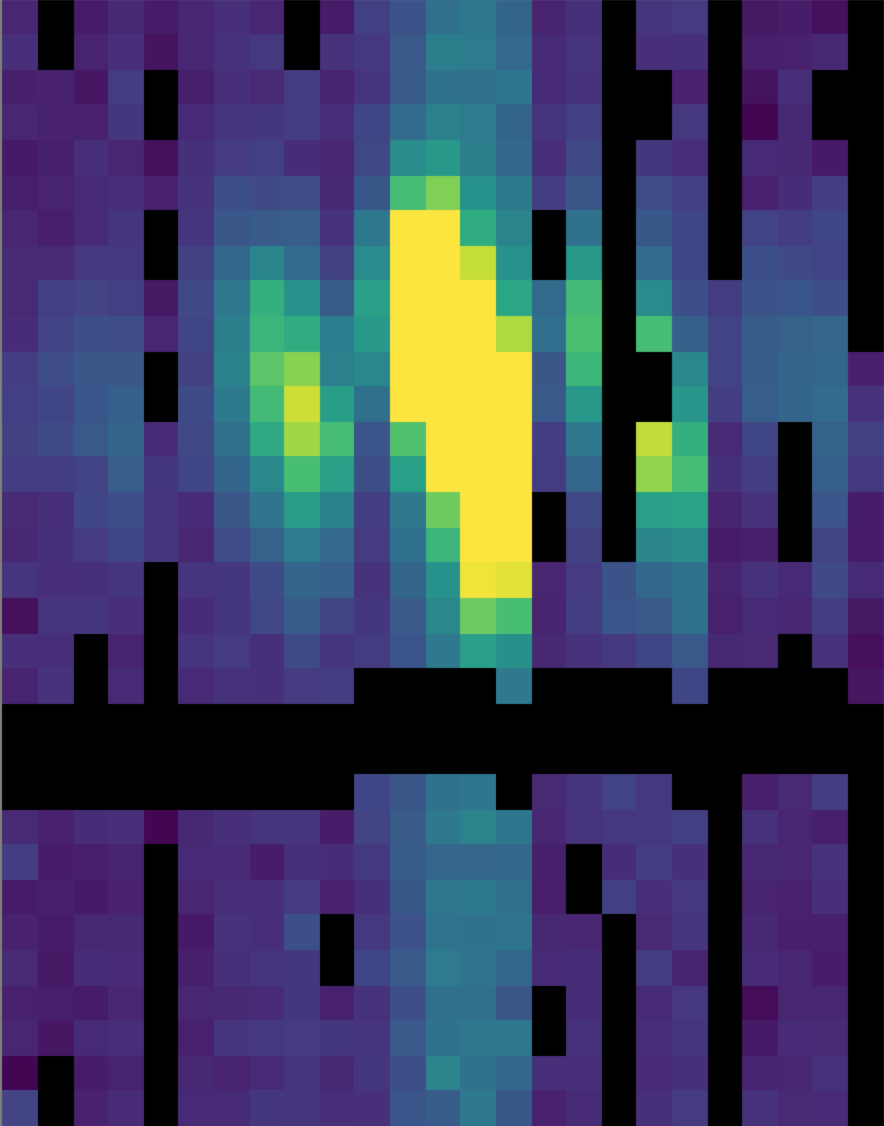
Fig. 30 The telluric-corrected flux array. Some pixels are set to NaN due to poor atmospheric transmission at those wavelengths. The cutoff level was set to 80% for this observation, for illustrative purposes.

Flux Calibrate

Flux calibration of FIFI-LS data is carried out via the division of the instrumental response, as recorded in response files appropriate for each grating setting, wavelength range, and dichroic. The response values have units of ADU/s/Hz/Jy and are derived from observations of “flux standards.” At the wavelengths at which FIFI-LS operates, there are very few stars bright enough to yield high signal-to-noise data useful for flux calibration purposes. Therefore, observations of asteroids, planets, and planetary moons are used, along with models of such objects, to derive the response curves. Since the observed fluxes of such solar system objects vary with time, the models must be generated for the time of each specific observation. To date, observations of Mars have been used as the primary flux calibration source. Predicted total fluxes for Mars across the FIFI-LS passband at the specific UT dates of the observations have been generated using the model of Lellouch and Amri. [1] Predicted fluxes at several frequencies have been computed and these have then been fit with blackbody curves to derive values at a large number of wavelength points. The deviations of the fits from the input predictions are much less than 1%. After the models have been generated, the telluric-corrected spectra of the standards, in units of ADU/s/Hz, are divided by the theoretical spectra, in Jy. The results are smoothed and then fit with a polynomial to derive response functions (ADU/s/Hz/Jy) that can then used to flux calibrate the telluric-corrected spectra of other astronomical sources (see Fig. 31).

[1]

See http://www.lesia.obspm.fr/perso/emmanuel-lellouch/mars/index.php

The pipeline stores a set of response functions for each channel and dichroic value. To perform flux calibration, it selects the correct response function for each input observation, interpolates the response onto the wavelengths of each spexel, and divides the flux by the response value to convert it to physical units (Jy/pixel). From this point on, the data products are considered to be Level 3 (FITS keyword PROCSTAT=LEVEL_3). For reference, the resampled response data is attached to the FITS file as a 25 x (16 * N_scan) data table in the first FITS extension (column RESPONSE). Flux calibration is applied to both the telluric-corrected cube and the uncorrected cube. The estimated systematic error in the flux calibration is recorded in the CALERR keyword in the FITS header, as an average fractional error. At this time, flux calibration is expected to be good to within about 5-10% (CALERR \(\leq\) 0.1). [2]

[2]

Earlier versions of this pipeline (prior to v1.3.2) propagated the systematic error on the flux calibration in the STDDEV and ERROR arrays in the output products. As of v1.3.2, the calibration error is only propagated in the FITS header keyword CALERR.

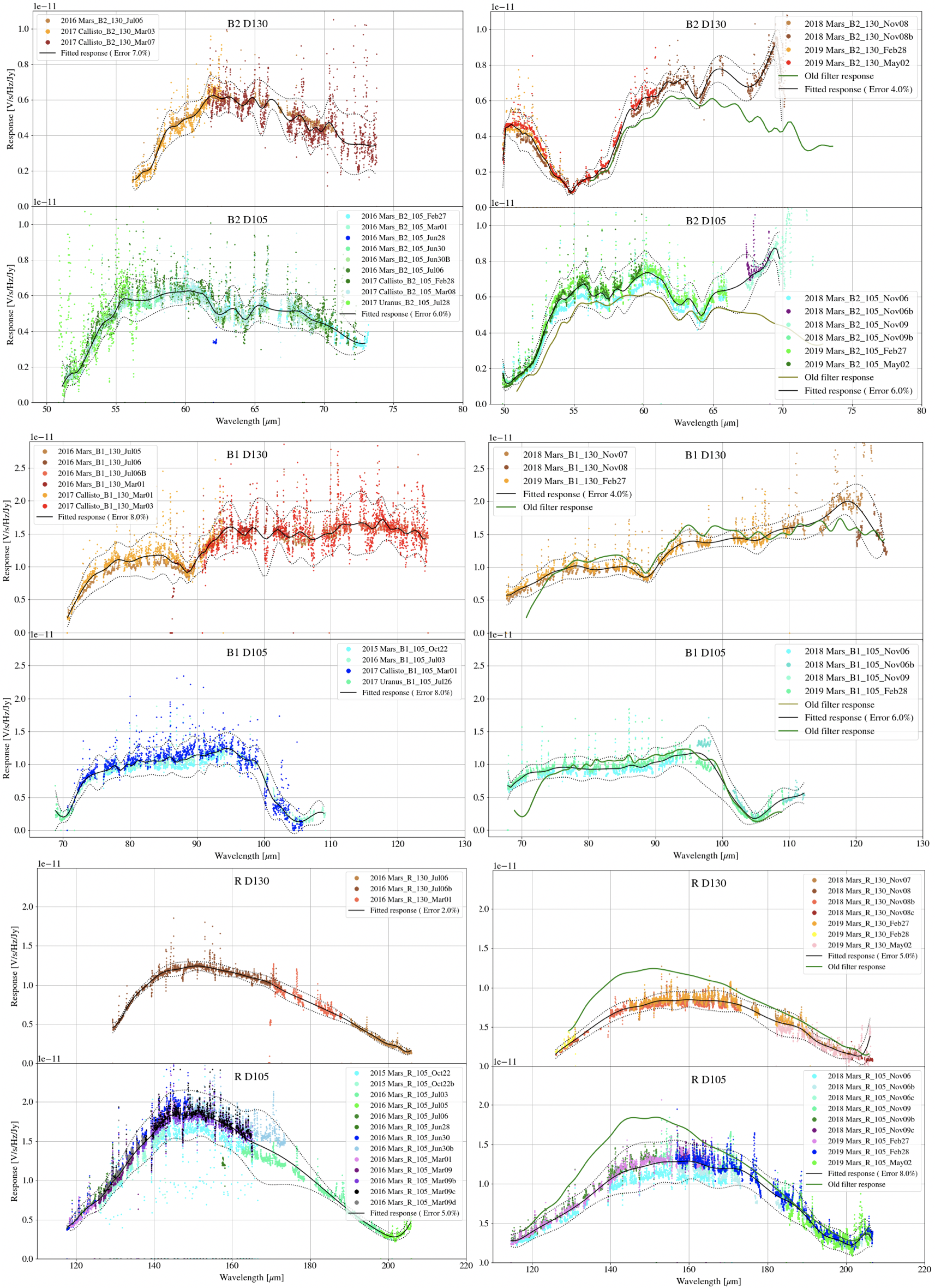
Fig. 31 Response fits overplotted on telluric-corrected data, with model spectra divided out. Data shown was taken in 2015-2019 for the blue channel order 2, blue channel order 1, and red channel. Plots on the left are from an older filter set; plots on the right are for data taken with an updated filter set.

Correct Wave Shift

Due to the motion of the Earth with respect to the barycenter of the solar system, the wavelengths of features in the spectra of astronomical sources will appear to be slightly shifted, by different amounts on different observation dates. In order to avoid introducing a broadening of spectral features when multiple observations obtained over different nights are combined, the wavelength calibration of FIFI-LS observations must be adjusted to remove the barycentric wavelength shift. This shift is calculated as an expected wavelength shift (\(d\lambda / \lambda\)), from the radial velocity of the earth with respect to the solar barycenter on the observation date, toward the RA and Dec of the observed target. This shift is recorded in the header keyword BARYSHFT, and applied to the wavelength calibration in the LAMBDA extension as:

\[\lambda' = \lambda + \lambda(d\lambda/\lambda)\]

Since the telluric absorption lines do not change with the motion of the earth, the barycentric wavelength shift cannot be applied to non-telluric-corrected data. Doing so would result in a spectrum in which both the intrinsic features and the telluric lines are shifted. Therefore, the unshifted wavelength calibration is also propagated in the output file, in the extension UNCORRECTED_LAMBDA.

It is possible to apply an additional wavelength shift to correct for the solar system’s velocity with respect to the local standard of rest (LSR). This shift is calculated and stored in the header keyword LSRSHFT, but it is not applied to the wavelength calibration. [3]

[3]

Earlier versions of this pipeline (prior to v2.4.0) applied both the barycentric shift and the shift to LSR to the wavelength calibration. The summed barycentric and LSR radial velocity was stored as the BARYSHFT value.

Resample

Finally, the pipeline resamples the flux for each spatial and spectral pixel onto a regular 3D grid (right ascension, declination, and wavelength). This step combines the spatial information from all input nod-combined dither positions into a single output map. See Fig. 32 for an overview of the resampling algorithm.

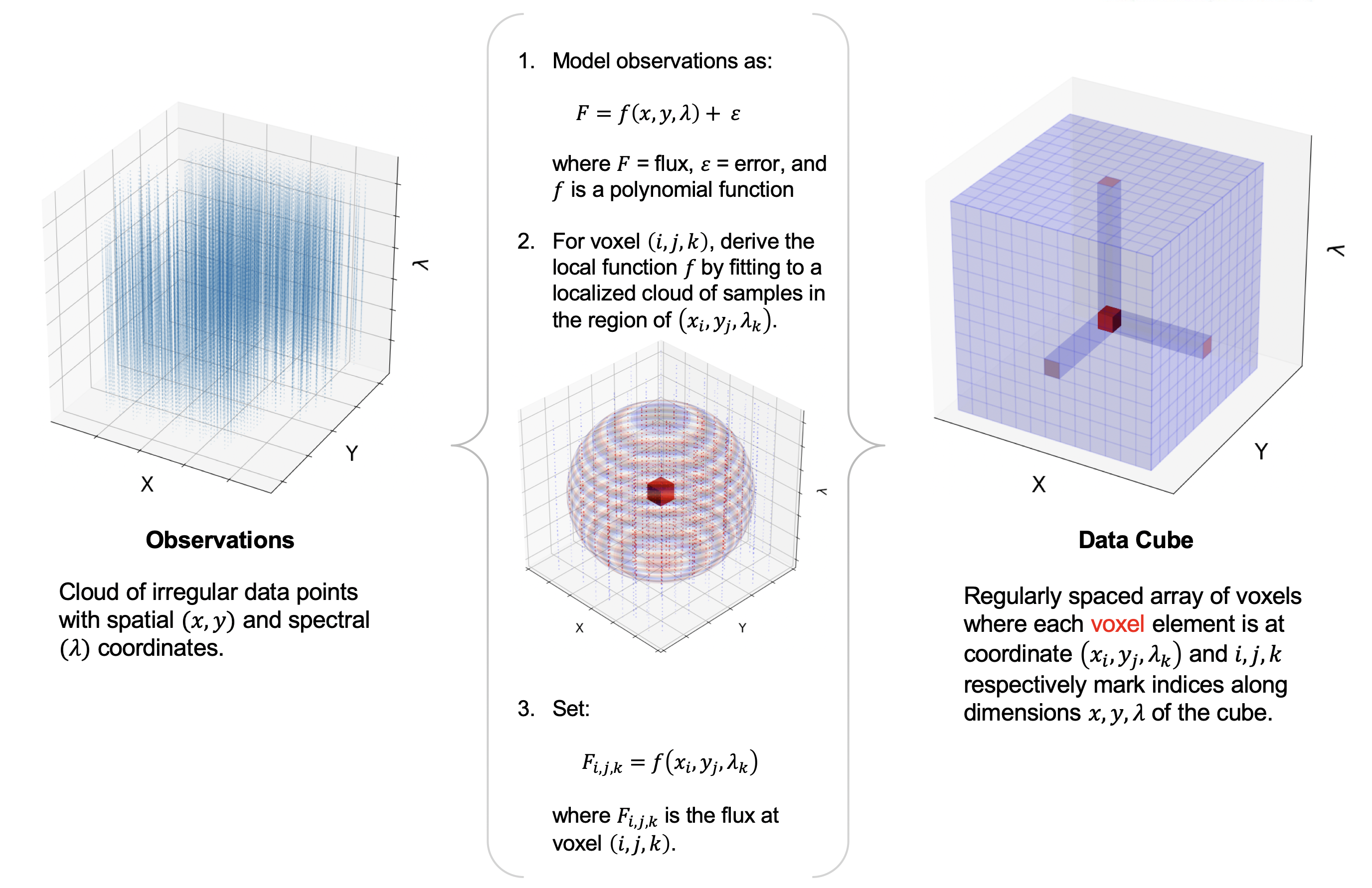
Fig. 32 Overview of the resampling algorithm. Given a cloud of irregularly spaced data points, the algorithm assigns values to voxels of a regular grid by fitting data points in a local cloud with a low-order polynomial function.

Grid Size

The pipeline first determines the maximum and minimum wavelengths and spatial offsets present in all input files by projecting all dither positions for the observation into a common world coordinate system (WCS) reference frame. For OTF data, the scan positions for each ramp in each input file are also considered. The full range of sky positions and wavelengths observed sets the range of the output grid.

The spacing of the output grid in the wavelength dimension (dw) is set by the desired oversampling. By default, in the wavelength dimension, the pipeline samples the average expected spectral FWHM for the observation (Table 5) with 8 output pixels.

The spacing in the spatial dimensions (dx) is fixed for each channel at 1.5 arcseconds in the BLUE and 3.0 arcseconds in the RED. These values are chosen to ensure an oversampling of the spatial FWHM by at least a factor of three.

For example, for the RED observation in the figures above, the expected spectral FWHM at the central wavelength is 0.13 um, so sampling this FWHM with 8 pixels creates a grid with a spectral width of 0.016 um. Given a min and max wavelength of 157.27 um and 158.48 um, the output grid will sample the full range of wavelengths with 76 spectral pixels. Since it is a RED channel observation, the spatial scale will be 3.0 arcseconds. If the range of x offsets is -41.0 to 57.74 and the range of y offsets is -43.9 to 36.9, then the output spatial grid will have dimensions 33 x 27, with an oversampling of the FWHM (using the interpolated value at 157.876 um of 15.6 arcseconds) of 5.2. The full output cube then is 33 x 27 x 76 (nx x ny x nw).

In the spatial dimensions, the flux in each pixel represents an integrated flux over the area of the pixel. Since the pixel width changes after resampling, the output flux must be corrected for flux conservation. To do so, the resampled flux is multiplied by the area of the new pixel (dx²), divided by the intrinsic area of the spaxel (approximately 36 arcseconds² for BLUE, 144 arcseconds² for RED).

Table 5 Spectral and spatial resolution by central wavelength

Channel/Order	Wavelength (um)	Spectral Resolution (\(d\lambda/\lambda\))	Spatial Resolution (arcsec)
Blue Order 1	70	545	6.9
Blue Order 1	80	570	7.9
Blue Order 1	90	628	8.9
Blue Order 1	100	720	9.9
Blue Order 1	110	846	11.0
Blue Order 1	120	1005	12.0
Blue Order 2	45	947	5.9
Blue Order 2	50	920	6.2
Blue Order 2	65	1415	7.3
Blue Order 2	70	1772	7.7
Red	120	747	11.9
Red	140	939	13.9
Red	160	1180	15.8
Red	180	1471	17.7
Red	200	1813	19.6

Algorithm

For each pixel in the 3D output grid, the resampling algorithm finds all flux values with assigned wavelengths and spatial positions within a fitting window, typically 0.5 times the spectral FWHM in the wavelength dimension, and 3 times the spatial FWHM in the spatial dimensions. For the spatial grid, a larger fit window is typically necessary than for the spectral grid, since the observation setup usually allows more oversampling in wavelength than in space.

Then, a low-order 3D polynomial surface is fit to all the good data points within the window. The fit is weighted by the error on the flux, as calculated by the pipeline, and a Gaussian function of the distance of the input data value from the grid location. The distance weighting function may be held constant for each output pixel, or it may optionally be allowed to vary in scale and shape in response to the input data characteristics. This adaptive smoothing kernel may help in preserving peak flux values for bright, compact flux regions, but may over-fit the input data in some sparsely sampled observations (see Fig. 33).

The output flux value for this algorithm is the value of the fit polynomial surface, evaluated at the grid location, and the associated error is the error on the fit (see Fig. 34).

Output grid locations for which there was insufficient input data for stable polynomial fits are set to NaN. The threshold for how much output data is considered invalid is a tunable parameter, but it is typically set to eliminate most edge effect artifacts from the final output cube.

For some types of observations, especially undithered observations of point sources for which the spatial FWHM is undersampled, the polynomial surface fits may not return good results. In these cases, it is beneficial to use an alternate resampling algorithm. In this algorithm, the master grid is determined as above, but each input file is resampled with polynomial fits in the wavelength dimension only. Then, for each wavelength plane, the spatial data is interpolated onto the grid, using radial basis function interpolation. Areas of the spatial grid for which there is no data in the input file are set to NaN. The interpolated cubes are then mean-combined, ignoring any NaNs, to produce the final output cube.

For either algorithm, the pipeline also generates an exposure map cube indicating the number of observations of the source that were taken at each pixel (see Fig. 35). These exposure counts correspond to the sum over the projection of the detector field of view for each input observation onto the output grid. The exposure map may not exactly match the valid data locations in the flux cube, since additional flagging and pixel rejection occurs during the resampling algorithms.

Uncorrected Flux Cube

Both the telluric-corrected and the uncorrected flux cubes are resampled in this step, onto the same 3D grid. However, the telluric-corrected cube is resampled using the wavelengths corrected for barycentric motion, and the uncorrected cube is resampled using the original wavelength calibration. The spectra from the uncorrected cube will appear slightly shifted with respect to the spectra from the telluric-corrected cube.

Detector Coordinates

For most observations, the output grid is determined from projected sky coordinates for each input data point, for the most accurate astrometry in the output map. However, this is undesirable for nonsidereal data, for which the sky coordinates of the target change over the course of the observation. For nonsidereal sources, the detector offsets (from input XS and YS extensions) are used instead of the sky coordinates (from RA and DEC extensions) to generate the output grid. For all other sources, detector coordinates may optionally be used instead of sky coordinates if desired.

Additional Scan Processing

For OTF data, the standard sky subtraction and flat correction algorithms may not be sufficient to remove residual sky and detector noise. In this mode, temporal variations frequently result in artifacts like striping along the scan direction, or residual sky backgrounds that overwhelm diffuse emission.

In this case, it may be beneficial to apply an iterative correction to the detector gain and noise. For OTF data, the FIFI-LS pipeline provides this correction as an optional scan reduction step, just prior to resampling. The iterative scan reduction algorithm is described at length in the HAWC+ pipeline user’s manual and in the software documentation for the sofia_redux.scan module.

At this time, this feature should be considered experimental. The scan algorithms have a number of complex, interlinked parameters that have not yet been fully tested and optimized for FIFI-LS data.

Output Data

The pipeline stores the resampled data as a 3D FITS image extension with extension name FLUX. The associated error is stored in a separate extension, with the name ERROR. The non-telluric-corrected cubes are stored in UNCORRECTED_FLUX and UNCORRECTED_ERROR extensions, respectively. The output wavelengths, x and y offsets, and RA and Dec coordinates are stored in WAVELENGTH, X, Y, RA—TAN, and DEC–TAN extensions.

For reference, a model of the atmospheric transmission spectrum, smoothed to the resolution of the observation, and the instrumental response curve used in flux calibration are also attached to the FITS file in 1D extensions called TRANSMISSION and RESPONSE.

Finally, an unsmoothed transmission spectrum is attached in a 2D image extension called UNSMOOTHED_TRANSMISSION. This extension will have size N_trans x 2, where N_trans is the number of data points in the spectrum, the first row is the wavelength array, and the second row is the transmission fraction. This spectrum may be useful for further analysis of the data (e.g. for determining the total flux in an emission line).

The final output from the pipeline is a FITS file with 11 image extensions:

• FLUX: The nx x ny x nw cube of flux values.

• ERROR: The associated error values on the flux (also nx x ny x nw).

• UNCORRECTED_FLUX: The nx x ny x nw cube of flux values that have not been corrected for atmospheric transmission.

• UNCORRECTED_ERROR: The associated error values on the uncorrected flux (also nx x ny x nw).

• WAVELENGTH: The wavelength values associated with each plane of the cube (nw).

• X: The x-coordinates of the data, in arcsecond offsets from the base position (nx).

• Y: The y-coordinates of the data, in arcsecond offsets from the base position (ny).

• RA—TAN: The right ascension coordinates of the data, in decimal hours, in a tangent projection from the base position.

• DEC–TAN: The declination coordinates of the data, in decimal degrees, in a tangent projection from the base position.

• TRANSMISSION: The atmospheric transmission model (nw).

• RESPONSE: The instrumental response curve (nw).

• EXPOSURE_MAP: The exposure map (nx x ny x nw).

• UNSMOOTHED_TRANSMISSION: The unsmoothed atmospheric transmission model (N_trans x 2).

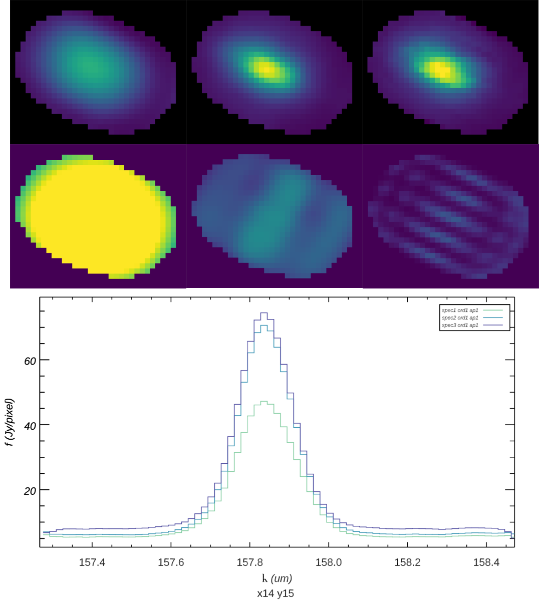
Fig. 33 Comparison of a non-adaptive (left), adaptively scaled (middle), and adaptively shaped and scaled (right) smoothing kernel for the above target, using a baseline smoothing radius corresponding to the spatial beam size. The top row shows the spatial slice at wavelength 157.83 um, locked to a common display scale. The bottom row shows the distance weights used by the resampling algorithm at the wavelength slice shown, also locked to a common display scale. Distance weights correlate with the size of the kernel used and the number of input pixels within the fit window. The plot below compares the spectral slice at pixel x,y = 14, 15 for the three resampled versions: green is non-adaptive, blue is adaptively scaled, and purple is adaptively shaped and scaled.

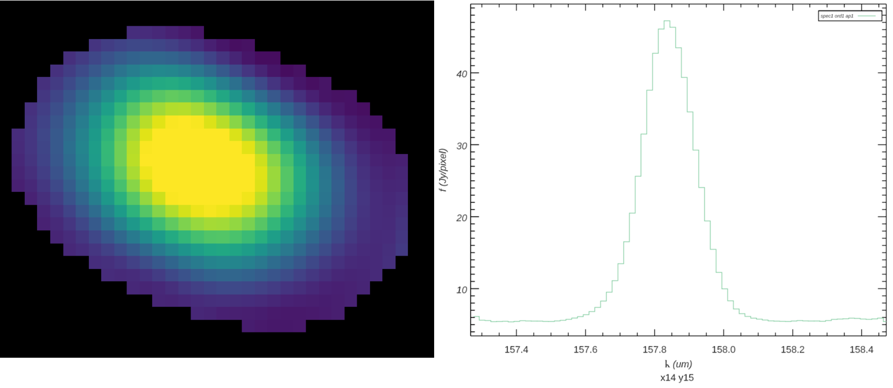
Fig. 34 The final output flux cube. The image on the left is a spatial slice at wavelength 157.83 um. The plot on the right is a spectral slice at pixel x,y = 14, 15, near the peak of the source.

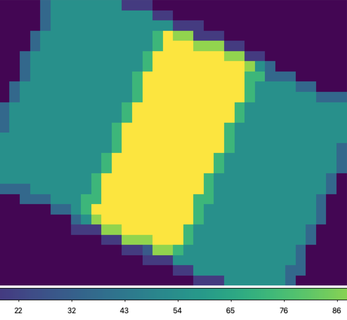
Fig. 35 Exposure map of input dither positions, corresponding to the above flux cube. Values range from 0 (purple, near the edges) to 108 (yellow, near the center).

Data products

Filenames

FIFI-LS output files from Redux are named according to the convention:

FILENAME = F####_FI_IFS_AOR-ID_CHANNEL_Type_FN1[-FN2].fits,

where #### is the four-digit SOFIA flight number, FI is the instrument identifier, IFS specifies that it is integral field spectroscopy data, AOR-ID is the AOR identifier for the observation, CHANNEL is either BLU or RED, Type is three letters identifying the product type (listed in the table below), and FN1 is the file number corresponding to the input file. FN1-FN2 is used if there are multiple input files for a single output file, where FN1 is the file number of the first input file and FN2 is the file number of the last input file.

Pipeline Products

The following table lists all intermediate products generated by Redux for FIFI-LS, in the order in which they are produced. The product type is stored in the primary FITS header of the file, under the keyword PRODTYPE. By default, the scan_combined, flux_calibrated, and and resampled products are saved. [4]

As a final step, the pipeline additionally produces an image in PNG format, intended to provide a quick-look preview of the data contained in the final product. These auxiliary products may be distributed to observers separately from the FITS file products.

[4]

Earlier versions of this pipeline (prior to v2.3.0) stored intermediate data as binary FITS tables, rather than image extensions. Refer to earlier revisions of this manual for more information.

Table 6 Final and intermediate data products

Step	Product Type	Proc. status	File code	Saved	Extensions
Split Grating / Chop	grating_chop_split	LEVEL_2	CP0, CP1	N	Nscan image extensions: FLUX_Gi for i=0…Nscan-1
Fit Ramps	ramps_fit	LEVEL_2	RP0, RP1	N	2 Nscan image extensions: FLUX_Gi, STDDEV_Gi for i=0…Nscan-1
Subtract Chops	chop_subtracted	LEVEL_2	CSB	N	2 Nscan image extensions: FLUX_Gi, STDDEV_Gi for i=0…Nscan-1
Combine Nods	nod_combined	LEVEL_2	NCM	N	2 Nscan image extensions: FLUX_Gi, STDDEV_Gi for i=0…Nscan-1
Lambda Calibrate	wavelength_calibrated	LEVEL_2	WAV	N	3 Nscan image extensions: FLUX_Gi, STDDEV_Gi, LAMBDA_Gi for i=0…Nscan-1
Spatial Calibrate	spatial_calibrated	LEVEL_2	XYC	N	5 Nscan image extensions: FLUX_Gi, STDDEV_Gi, LAMBDA_Gi XS_Gi, YS_Gi, RA_Gi, DEC_Gi for i=0…Nscan-1
Apply Flat	flat_fielded	LEVEL_2	FLF	N	7 Nscan image extensions: FLUX_Gi, STDDEV_Gi, LAMBDA_Gi XS_Gi, YS_Gi, RA_Gi, DEC_Gi, FLAT_Gi, FLATERR_Gi for i=0…Nscan-1
Combine Scans	scan_combined	LEVEL_2	SCM	Y	7 image extensions: FLUX, STDDEV, LAMBDA, XS, YS, RA, DEC
Telluric Correct	telluric_corrected	LEVEL_2	TEL	N	11 image extensions: FLUX, STDDEV, UNCORRECTED_FLUX, UNCORRECTED_STDDEV, LAMBDA, XS, YS, RA, DEC, ATRAN, UNSMOOTHED_ATRAN
Flux Calibrate	flux_calibrated	LEVEL_3	CAL	Y	12 image extensions: FLUX, STDDEV, UNCORRECTED_FLUX, UNCORRECTED_STDDEV, LAMBDA, XS, YS, RA, DEC, ATRAN, RESPONSE, UNSMOOTHED_ATRAN
Correct Wave Shift	wavelength_shifted	LEVEL_3	WSH	N	13 image extensions: FLUX, STDDEV, UNCORRECTED_FLUX, UNCORRECTED_STDDEV, LAMBDA, UNCORRECTED_LAMBDA, XS, YS, RA, DEC, ATRAN, RESPONSE, UNSMOOTHED_ATRAN
Spatial Resample	resampled	LEVEL_4	WXY	Y	13 image extensions: FLUX, ERROR, UNCORRECTED_FLUX, UNCORRECTED_ERROR, WAVELENGTH, X, Y, RA—TAN, DEC–TAN, TRANSMISSION, RESPONSE, EXPOSURE_MAP, UNSMOOTHED_TRANSMISSION

Data Format

All files produced by the pipeline are multi-extension FITS files, for which the primary HDU contains only the primary header, and all data is contained in separate extensions.

For standard chop/nod modes, all output extensions are FITS image extensions. Pipeline steps prior to the Combine Scans step output one extension of each type for each of N_scan grating scans performed. Intermediate flux and error data for all steps after the Fit Ramps step are 2D arrays (spaxel x spexel); the final product contains 3D spectral cubes (RA x Dec x wavelength).

For the OTF mode, intermediate data files produced by pipeline steps prior to the Spatial Calibrate step additionally contain a binary table holding sky position data for each scan position (extension SCANPOS_G0). Intermediate flux and error data in this mode are 3D cubes (spaxel x spexel x scan position). The final product is identical to other modes.

Grouping LEVEL_1 data for processing

FIFI-LS observations of a single object may dither in wavelength and/or in space. It is common to use a set of FIFI-LS observations to map out large regions of diffuse emission in a few small wavelength regions, but it is also common to use FIFI-LS to take a set of observations of a compact source over a wide range of wavelengths. As such, observations cannot simply be split on the central wavelength, or the base positions of the observation. Grouping relies on a keyword, FILEGPID, which defines a set of observations that should be reduced together to produce one final spectral map. In addition, however, observations must always be separated by detector channel, dichroic setting, nodding style (symmetric vs. asymmetric), observation type (source vs. sky flat), and the observational program ID. It may also be desirable to group file by the observation ID (AOR-ID), but this is considered optional. This is due to the fact that, because FIFI-LS incorporates a dichroic, different AORs can have the same grating setting for one of the two detectors. In such cases, the data sets with the same settings should be combined even though the AORs are different. All of these requirements together define a set of FITS keywords that must match in order for a group of input files to be reduced together (see Table 7).

Table 7 Grouping criteria

Keyword	Data Type	Match Criterion
OBSTYPE	STR	Exact
DETCHAN	STR	Exact
DICHROIC	INT	Exact
NODSTYLE	STR	Exact
PLANID	STR	Exact
FILEGPID	STR	Exact
AOR-ID (optional)	STR	Exact

Configuration and execution

Installation

The FIFI-LS pipeline is written entirely in Python. The pipeline is platform independent, but has been tested only on Linux and Mac OS X operating systems. Running the pipeline requires a minimum of 16GB RAM, or equivalent-sized swap file.

The pipeline is primarily comprised of four modules within the sofia_redux package: sofia_redux.instruments.fifi_ls, sofia_redux.pipeline, sofia_redux.spectroscopy, and sofia_redux.toolkit. Additional optional features are provided by the sofia_redux.calibration and sofia_redux.scan modules.

The fifi_ls module provides the data processing algorithms, with supporting libraries from the toolkit and spectroscopy modules. The pipeline module provides interactive and batch interfaces to the pipeline algorithms. The calibration module is used to provide interactive photometry routines in the interactive interface. The scan module provides support for additional processing tasks specific to on-the-fly mapping modes.

External Requirements

To run the pipeline for any mode, Python 3.8 or higher is required, as well as the following packages: numpy, scipy, matplotlib, pandas, astropy, configobj, numba, bottleneck, joblib, and astropy-helpers. Some display functions for the graphical user interface (GUI) additionally require the PyQt5, pyds9, photutils, and dill packages. All required external packages are available to install via the pip or conda package managers. See the Anaconda environment file (environment.yml), or the pip requirements file (requirements.txt) distributed with sofia_redux for specific version requirements.

Running the pipeline interactively also requires an installation of SAO DS9 for FITS image display. See http://ds9.si.edu/ for download and installation instructions. The ds9 executable must be available in the PATH environment variable for the pyds9 interface to be able to find and control it.

Source Code Installation

The source code for the FIFI-LS pipeline maintained by the SOFIA Data Processing Systems (DPS) team can be obtained directly from the DPS, or from the external GitHub repository. This repository contains all needed configuration files, auxiliary files, and Python code to run the pipeline on FIFI-LS data in any observation mode.

After obtaining the source code, install the four Python libraries with the command:

python setup.py install

from the top-level directory.

Alternately, a development installation may be performed from inside the directory with the command:

pip install -e .

After installation, the top-level pipeline interface commands should be available in the PATH. Typing:

redux

from the command line should launch the GUI interface, and:

redux_pipe -h

should display a brief help message for the command line interface.

Configuration

For FIFI-LS algorithms, default parameter values are defined by the Redux object that interfaces to them. These values may be overridden manually for each step, while running in interactive mode. They may also be overridden by an input parameter file, in INI format, in either interactive or automatic mode. See Appendix A for an example of an input parameter file, which contains the current defaults for all parameters.

Requirements for input header keywords are also specified in a configuration file, called headerdef.dat, located in the fifi_ls/data package directory. This table lists the keyword name, whether it is a value required to be present in the input headers, its default value, the data type of the value, and any requirements on the value range (minimum value, maximum value, or enumerated value). The table also defines how keywords from multiple input files should be combined for a single output file (e.g. take the first value, take the sum, string-concatenate, etc.). A sample of this configuration file is also given in Appendix A. All keywords present in the table will be written to output files produced by the FIFI-LS Redux pipeline.

Input data

Redux takes as input raw FIFI-LS FITS data files, which contain unsigned tables. The number of frames per raw data cube depends on the readout mode used to acquire the data. The FITS headers contain data acquisition and observation parameters and, combined with the pipeline configuration files, comprise the information necessary to complete all steps of the data reduction process. Some critical keywords are required to be present in the raw data in order to perform a successful grouping, reduction, and ingestion into the SOFIA archive (see Appendix A).

It is assumed that the input data have been successfully grouped before beginning reduction: Redux considers all input files in a reduction to be science files that are part of a single homogeneous reduction group, to be reduced together with the same parameters.

Auxiliary Files

In order to complete a standard reduction, the pipeline requires a number of auxiliary files to be on disk, in standard locations within the fifi_ls/data package directory. These files may be overridden in custom reductions, using input parameters for the relevant pipeline steps. See Table 8 for a table of all commonly used types of auxiliary files.

Table 8 Auxiliary files used by FIFI-LS reductions

Auxiliary File	File Type	Pipe Step	Comments
Bad Pixel	ASCII	Fit Ramps	Contains a list of known bad pixels
Wavelength Calibration	CSV	Lambda Calibrate	Contains wavelength calibration constants, by date
Spatial Calibration	ASCII	Spatial Calibrate	Contains spaxel position values, by date
Spatial Flat	ASCII	Apply Flat	Contains flat correction values for all 25 spaxels, by date
Spectral Flat	FITS	Apply Flat	Contains flat correction values for all spexels at all possible wavelengths
Resolution	ASCII	Telluric Correct, Resample	Contains the expected spatial and spectral resolution for all modes
ATRAN	FITS	Telluric Correct	Contains an unsmoothed atmospheric transmission model spectrum
Response	FITS	Flux Calibrate	Contains an instrumental response spectrum

Automatic Mode Execution

The DPS pipeline infrastructure runs a pipeline on previously-defined reduction groups as a fully-automatic black box. To do so, it creates an input manifest (infiles.txt) that contains relative paths to the input files (one per line). The command-line interface to the pipeline is run as:

redux_pipe infiles.txt

The command-line interface will read in the specified input files, use their headers to determine the observation mode, and accordingly the steps to run and any intermediate files to save. Output files are written to the current directory, from which the pipeline was called. After reduction is complete, the script will generate an output manifest (outfiles.txt) containing the relative paths to all output FITS files generated by the pipeline.

Optionally, in place of a manifest file, file paths to input files may be directly specified on the command line. Input files may be raw FITS files, or may be intermediate products previously produced by the pipeline. For example, this command will complete the reduction for a set of FITS files in the current directory, previously reduced through the calibration step of the pipeline:

redux_pipe *CAL*.fits

To customize batch reductions from the command line, the redux_pipe interface accepts a configuration file on the command line. This file may contain any subset of the full configuration file, specifying any non-default parameters for pipeline steps. An output directory for pipeline products and the terminal log level may also be set on the command line.

The full set of optional command-line parameters accepted by the redux_pipe interface are:

-h, --help            show this help message and exit
-c CONFIG, --configuration CONFIG
                      Path to Redux configuration file.
-o OUTDIR, --out OUTDIR
                      Path to output directory.
-l LOGLEVEL, --loglevel LOGLEVEL
                      Log level.

Manual Mode Execution

In manual mode, the pipeline may be run interactively, via a graphical user interface (GUI) provided by the Redux package. The GUI is launched by the command:

redux

entered at the terminal prompt (Fig. 36). The GUI allows output directory specification, but it may write initial or temporary files to the current directory, so it is recommended to start the interface from a location to which the user has write privileges.

From the command line, the redux interface accepts an optional config file (-c) or log level specification (-l), in the same way the redux_pipe command does. Any pipeline parameters provided to the interface in a configuration file will be used to set default values; they will still be editable from the GUI.

Fig. 36 Redux GUI startup.

Basic Workflow

To start an interactive reduction, select a set of input files, using the File menu (File->Open New Reduction). This will bring up a file dialog window (see Fig. 37). All files selected will be reduced together as a single reduction set.

Redux will decide the appropriate reduction steps from the input files, and load them into the GUI, as in Fig. 38.

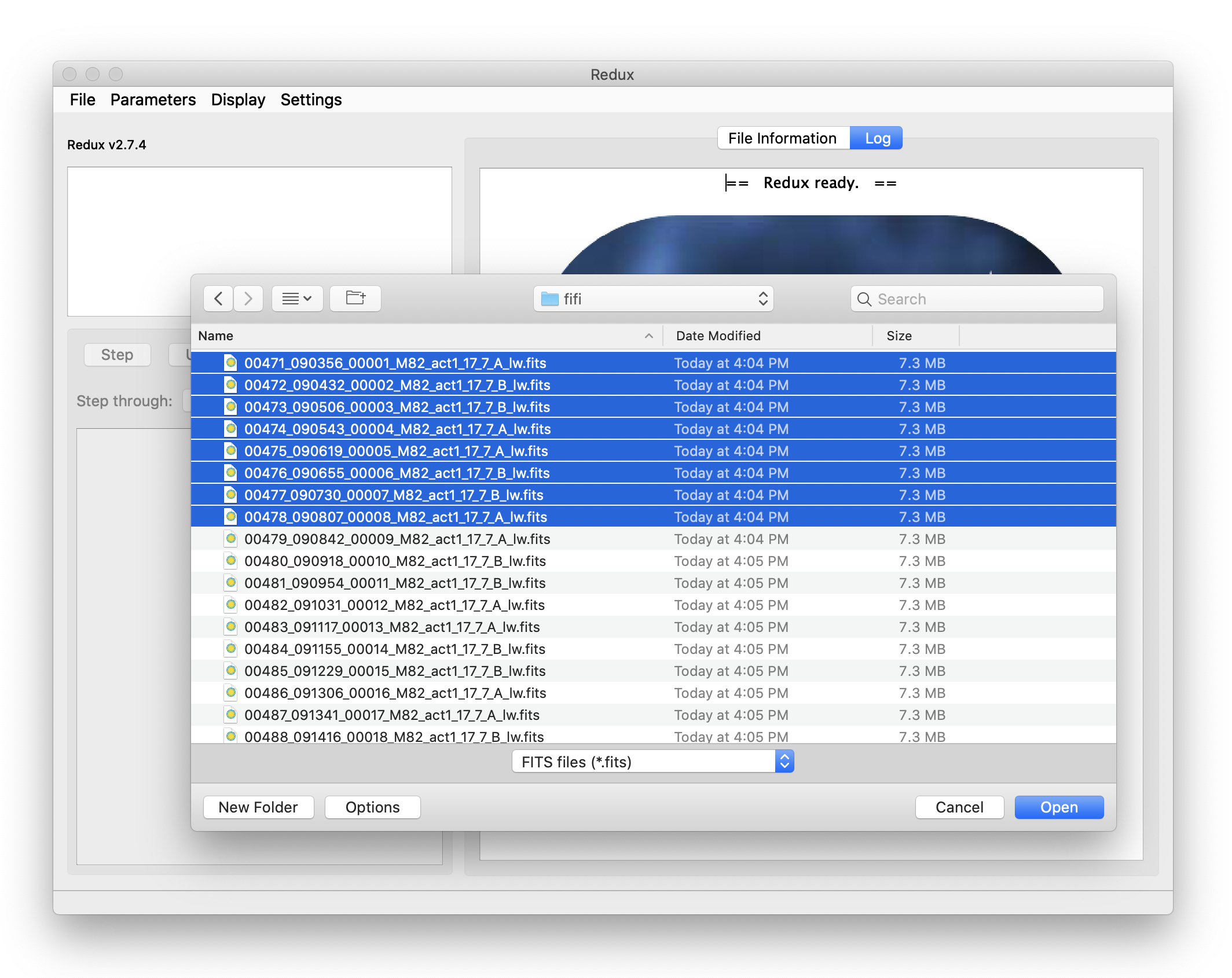
Fig. 37 Open new reduction.

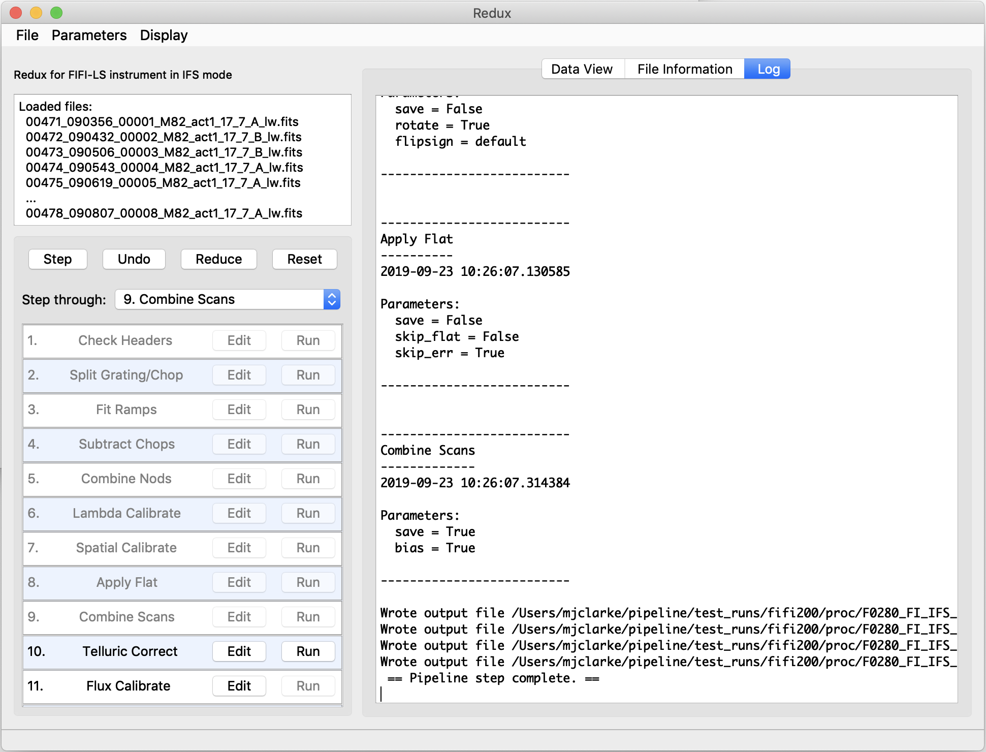
Fig. 38 Sample reduction steps. Log output from the pipeline is displayed in the Log tab.

Each reduction step has a number of parameters that can be edited before running the step. To examine or edit these parameters, click the Edit button next to the step name to bring up the parameter editor for that step (Fig. 39). Within the parameter editor, all values may be edited. Click OK to save the edited values and close the window. Click Reset to restore any edited values to their last saved values. Click Restore Defaults to reset all values to their stored defaults. Click Cancel to discard all changes to the parameters and close the editor window.

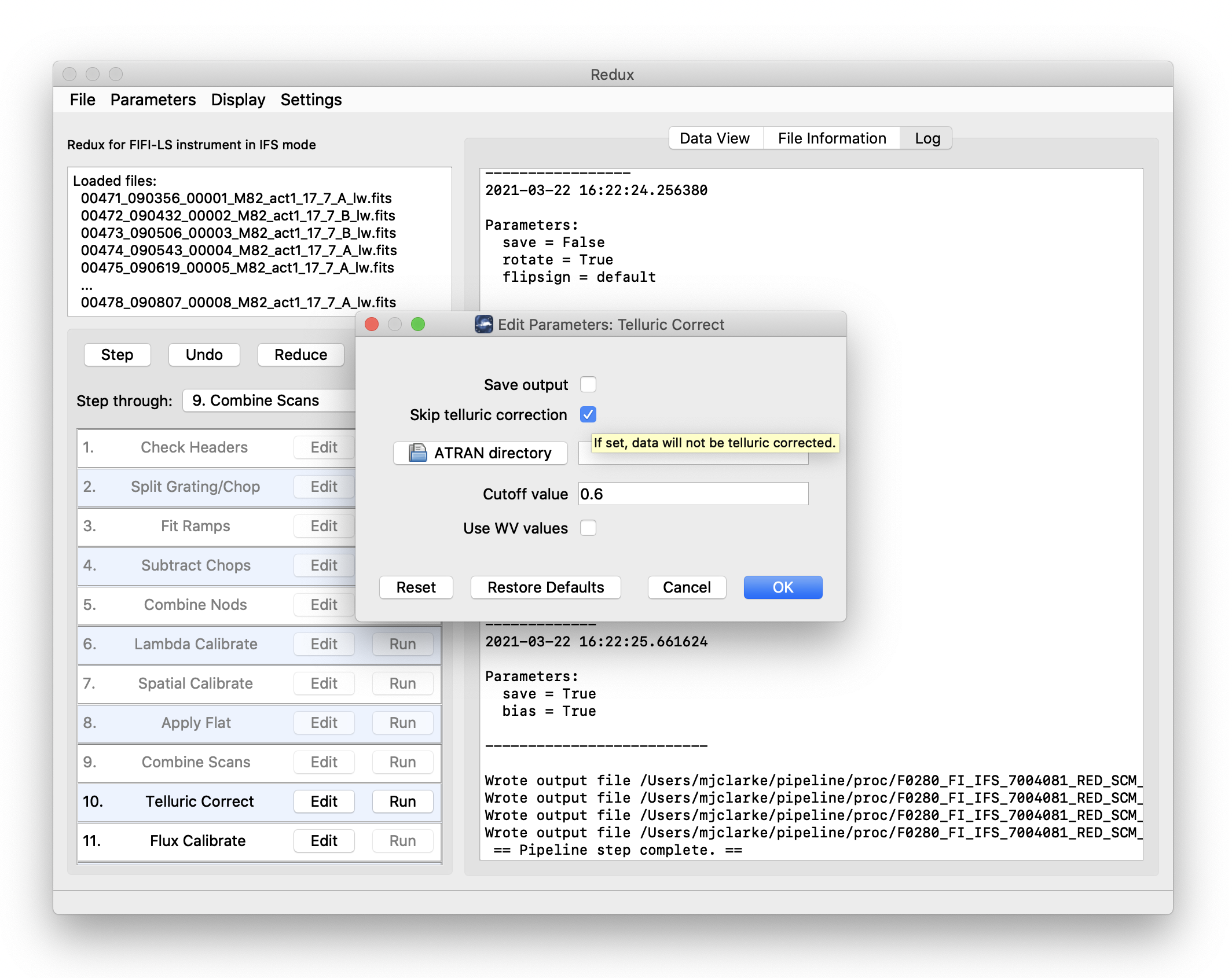
Fig. 39 Sample parameter editor for a pipeline step.

The current set of parameters can be displayed, saved to a file, or reset all at once using the Parameters menu. A previously saved set of parameters can also be restored for use with the current reduction (Parameters -> Load Parameters).

After all parameters for a step have been examined and set to the user’s satisfaction, a processing step can be run on all loaded files either by clicking Step, or the Run button next to the step name. Each processing step must be run in order, but if a processing step is selected in the Step through: widget, then clicking Step will treat all steps up through the selected step as a single step and run them all at once. When a step has been completed, its buttons will be grayed out and inaccessible. It is possible to undo one previous step by clicking Undo. All remaining steps can be run at once by clicking Reduce. After each step, the results of the processing may be displayed in a data viewer. After running a pipeline step or reduction, click Reset to restore the reduction to the initial state, without resetting parameter values.

Files can be added to the reduction set (File -> Add Files) or removed from the reduction set (File -> Remove Files), but either action will reset the reduction for all loaded files. Select the File Information tab to display a table of information about the currently loaded files (Fig. 40).

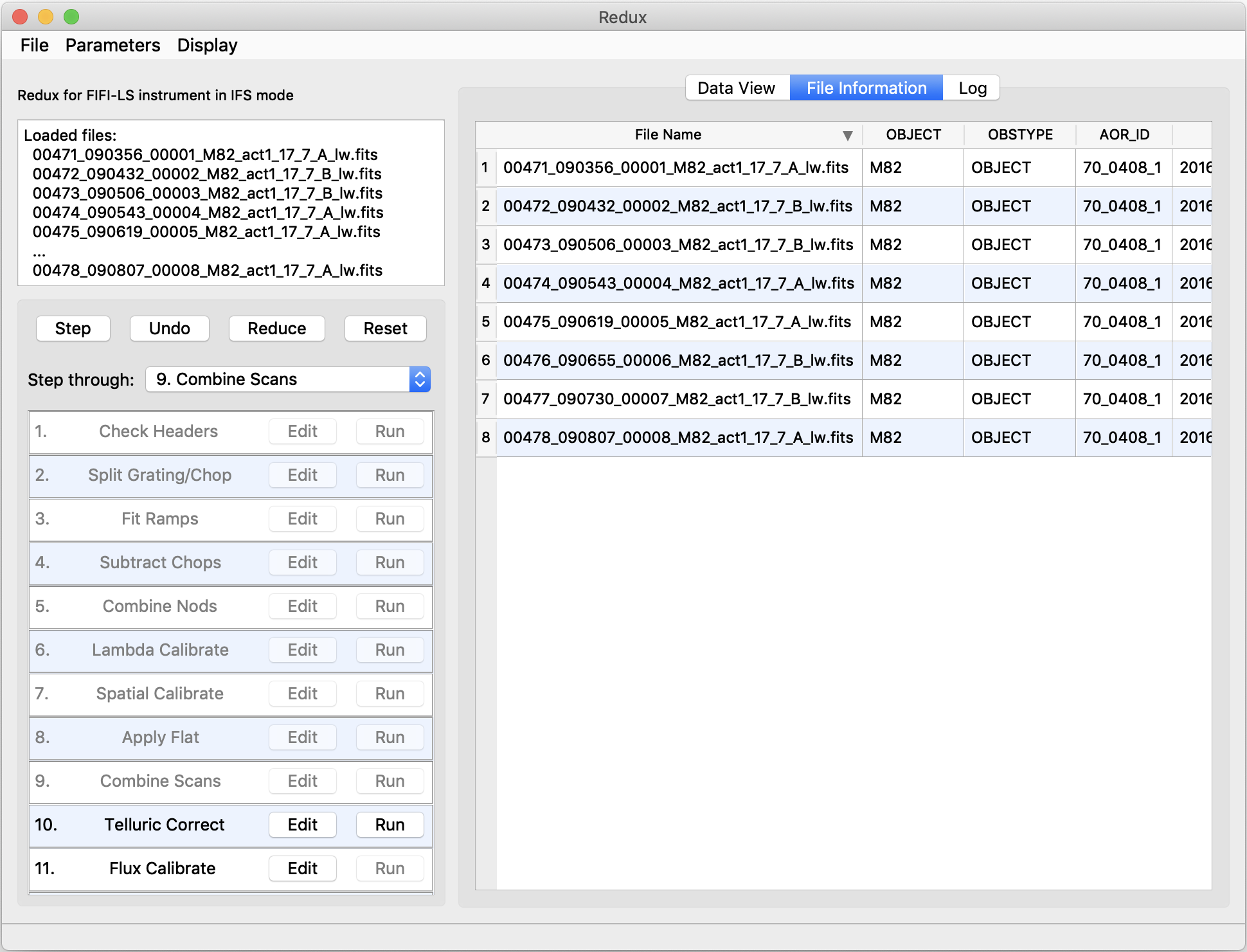
Fig. 40 File information table.

Display Features

The Redux GUI displays images for quality analysis and display (QAD) in the DS9 FITS viewer. DS9 is a standalone image display tool with an extensive feature set. See the SAO DS9 site (http://ds9.si.edu/) for more usage information.

After each pipeline step completes, Redux may load the produced images into DS9. Some display options may be customized directly in DS9; some commonly used options are accessible from the Redux interface, in the Data View tab (Fig. 41).

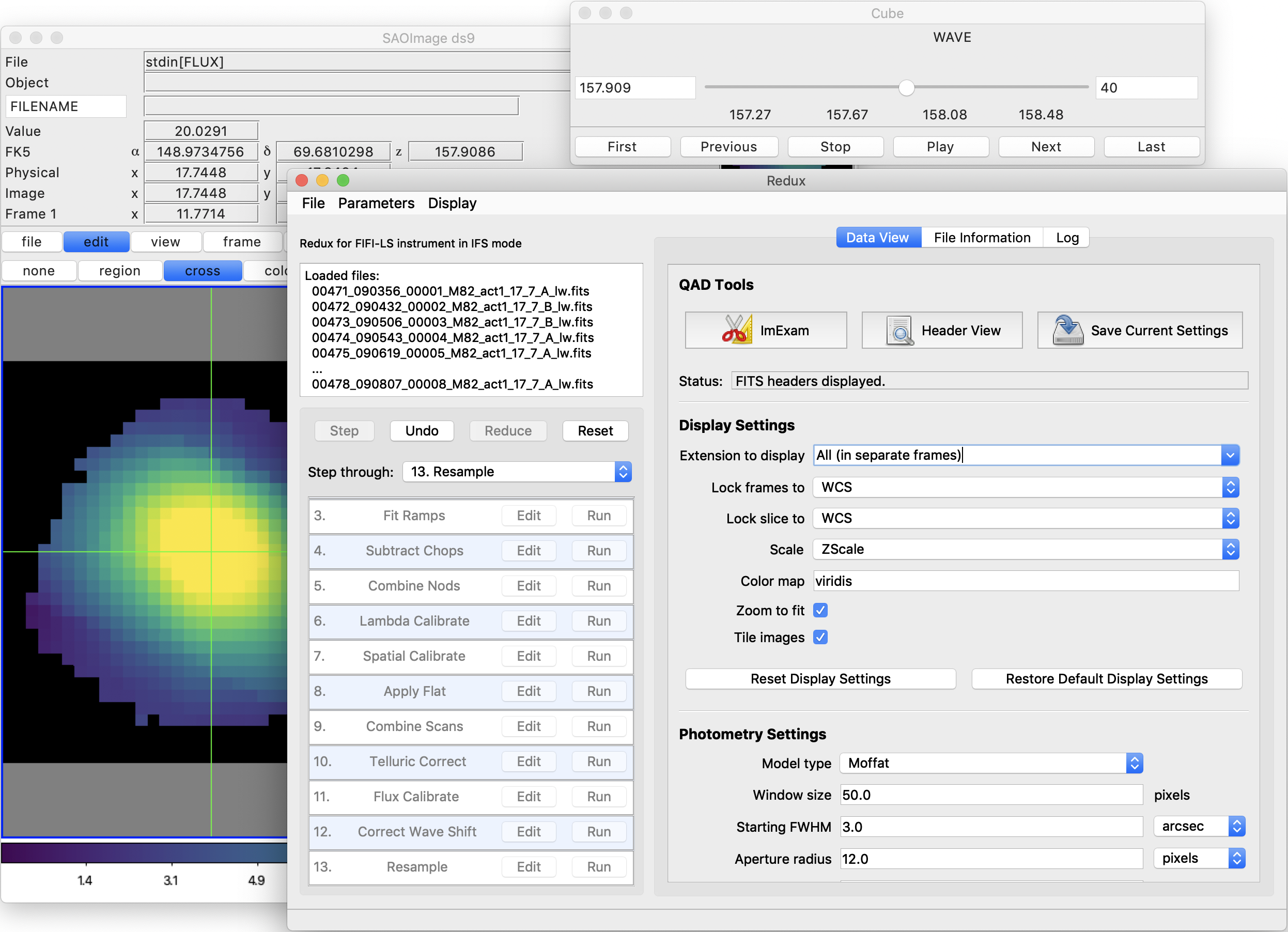
Fig. 41 Data viewer settings and tools.

From the Redux interface, the Display Settings can be used to:

• Set the FITS extension to display (First, or edit to enter a specific extension), or specify that all extensions should be displayed in a cube or in separate frames.

• Lock individual frames together, in image or WCS coordinates.

• Lock cube slices for separate frames together, in image or WCS coordinates.

• Set the image scaling scheme.

• Set a default color map.

• Zoom to fit image after loading.

• Tile image frames, rather than displaying a single frame at a time.

Changing any of these options in the Data View tab will cause the currently displayed data to be reloaded, with the new options. Clicking Reset Display Settings will revert any edited options to the last saved values. Clicking Restore Default Display Settings will revert all options to their default values.

In the QAD Tools section of the Data View tab, there are several additional tools available.

Clicking the ImExam button (scissors icon) launches an event loop in DS9. After launching it, bring the DS9 window forward, then use the keyboard to perform interactive analysis tasks:

• Type ‘a’ over a source in the image to perform photometry at the cursor location.

• Type ‘p’ to plot a pixel-to-pixel comparison of all frames at the cursor location.

• Type ‘s’ to compute statistics and plot a histogram of the data at the cursor location.

• Type ‘c’ to clear any previous photometry results or active plots.

• Type ‘h’ to print a help message.

• Type ‘q’ to quit the ImExam loop.

The photometry settings (the image window considered, the model fit, the aperture sizes, etc.) may be customized in the Photometry Settings. Plot settings (analysis window size, shared plot axes, etc.) may be customized in the Plot Settings. After modifying these settings, they will take effect only for new apertures or plots (use ‘c’ to clear old ones first). As for the display settings, the reset button will revert to the last saved values and the restore button will revert to default values. For the pixel-to-pixel and histogram plots, if the cursor is contained within a previously defined DS9 region (and the regions package is installed), the plot will consider only pixels within the region. Otherwise, a window around the cursor is used to generate the plot data. Setting the window to a blank value in the plot settings will use the entire image.

Clicking the Header button (magnifying glass icon) from the QAD Tools section opens a new window that displays headers from currently loaded FITS files in text form (Fig. 42). The extensions displayed depends on the extension setting selected (in Extension to Display). If a particular extension is selected, only that header will be displayed. If all extensions are selected (either for cube or multi-frame display), all extension headers will be displayed. The buttons at the bottom of the window may be used to find or filter the header text, or generate a table of header keywords. For filter or table display, a comma-separated list of keys may be entered in the text box.

Clicking the Save Current Settings button (disk icon) from the QAD Tools section saves all current display and photometry settings for the current user. This allows the user’s settings to persist across new Redux reductions, and to be loaded when Redux next starts up.

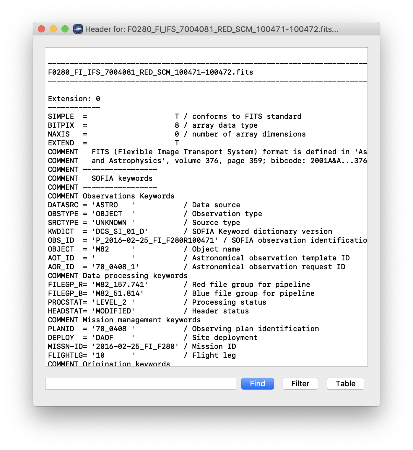
Fig. 42 QAD FITS header viewer.

FIFI-LS Reduction

FIFI-LS data reduction with Redux follows the data reduction flowchart given in Fig. 22. At each step, Redux attempts to determine automatically the correct action, given the input data and default parameters, but each step can be customized as needed.

Some key parameters to note are listed below.

• Check Headers

  • Abort reduction for invalid headers: By default, Redux will halt the reduction if the input header keywords do not meet requirements. Uncheck this box to attempt the reduction anyway.

• Fit Ramps

  • Signal-to-noise threshold: This value defines the signal-to-noise cut-off to flag a ramp as bad and ignore it. Set to -1 to skip the signal-to-noise cut.

  • Combination threshold (sigma): This value defines the rejection threshold for the robust mean combination of the ramp slopes. Set higher to reject fewer ramps, lower to reject more.

  • Bad pixel file: By default, the pipeline looks up a bad pixel mask in fifi-ls/data/badpix_files. To override the default mask, use this parameter to select a different text file. The file must be an ASCII table with two columns: the spaxel number (1-25, numbered left to right in displayed array), and the spexel number (1-16, numbered bottom to top in displayed array). This option may be used to block a bad spaxel for a particular observation, by entering a bad pixel for every spexel index in a particular spaxel.

  • Remove 1st 2 ramps: Select to remove the first two ramps. This is on by default. This option has no effect if there are fewer than three ramps per chop.

  • Subtract bias: If set, the value from the open zeroth spexel will be subtracted before fitting.

  • Threshold for grating instability: Threshold in sigma for allowed ramp-averaged deviation from the expected grating position. Set to -1 to turn off filtering.

• Combine Nods

  • Method for combining off-beam images: For C2NC2 only: ‘nearest’ takes the closest B nod in time, ‘average’ will mean-combine before and after B nods, and ‘interpolate’ will linearly interpolate before and after B nods to the A nod time. For OTF mode data, the B nods are interpolated to the time of each scan position.

  • Propagate off-beam image instead of on-beam: If selected, B beams will be treated as if they were A beams for all subsequent reductions. That is, the map will be produced at the B position instead of the A. All other filenames and header settings will remain the same, so use with caution. This option is mostly used for testing purposes.

• Spatial Calibrate

  • Rotate by detector angle: By default, Redux rotates the data by the detector angle to set North up and East to the left in the final map. Deselect this box to keep the final map in detector coordinates.

  • Flip RA/Dec sign convention (+, -, or default): For most data, the sign convention of the DLAM_MAP and DBET_MAP header keywords, which define the dither offsets, is determined automatically (parameter value “default”). Occasionally, for particular observations, these keywords may need their signs flipped, or used as is (no flip). This is usually determined by inspection of the results of the Resample step.

• Apply Flat

  • Skip flat correction: Select this option to skip flat-fielding the data. This option is mostly used for testing purposes.

  • Skip flat error propagation: Deselect this option to propagate the systematic flat correction error in the flux error plane. This option is not currently recommended: the systematic error is stored in the CALERR keyword instead.

• Combine Scans

  • Correct bias offset: Select this option to subtract an overall bias offset between the individual grating scans.

• Telluric Correct

  • Skip telluric correction: Select to skip correcting the data for telluric absorption. This option is mostly used for testing.

  • ATRAN directory: Use this option to select a directory containing ATRAN FITS files. This must be set in order to use water vapor values for telluric correction.

  • Cutoff value: Modify to adjust the transmission fraction below which the telluric-corrected data will be set to NaN.

  • Use WV values: Select to use water vapor values from the header (keyword WVZ_OBS) to select the ATRAN file to apply. This option will have no effect unless the ATRAN directory is set to a location containing ATRAN files derived for different PWV values.

• Flux Calibrate

  • Skip flux calibration: Select to skip flux calibration of the data. The flux will remain in instrumental units (ADU/sec), with PROCSTAT=LEVEL_2. This option is mostly used for testing.

  • Response file: Use this option to select a FITS file containing an instrumental response spectrum to use in place of the default file on disk.

• Correct Wave Shift

  • Skip wavelength shift correction: Select to skip applying the correction to the wavelength calibration due to barycentric velocity. In this case, both telluric-corrected and uncorrected cubes will be resampled onto the original wavelengths. This option is mostly used for testing.

• Resample

  • General parameters

    • Use parallel processing: If not set, data will be processed serially. This will likely result in longer processing times, but smaller memory footprint during processing.

    • Maximum cores to use: Specify the maximum cores to use, in the case of parallel processing. If not specified, the maximum is the number of available cores, minus 1.

    • Check memory use during resampling: If set, memory availability will be checked before processing, and the number of processes will be modified if necessary. If not set, processing is attempted with the maximum number of cores specified. Use with caution: in some conditions, unsetting this option may result in software or computer crashes.

    • Skip coadd: If selected, a separate flux cube will be made from each input file, using the interpolation algorithm. This option is useful for identifying bad input files.

    • Interpolate instead of fit: If set, an alternate resampling algorithm will be used, rather than the local polynomial surface fits. This option may be preferable for data with small dither offsets; it is not recommended for large maps.

    • Weight by errors: If set, local fits will be weighted by the flux errors, as calculated by the pipeline.

    • Fit rejection threshold (sigma): If the fit value is more than this number times the standard deviation away from the weighted mean, the weighted mean is used instead of the fit value. This parameter is used to reject bad fit values. Set to -1 to turn off.

    • Positive outlier threshold (sigma): Sets the rejection threshold for the input data, in sigma. Set to -1 to turn off.

    • Negative outlier threshold (sigma): If non-zero, sets a separate rejection threshold in sigma for negative fluxes, to be used in a first-pass rejection. Set to -1 to turn off.

    • Append distance weights to output file: If set, distance weights calculated by the resampling algorithm will be appended to the output FITS file. This option is primarily used for testing.

    • Skip computing the uncorrected flux cube: If set, the uncorrected flux data will be ignored. This option is primarily for faster testing and/or quicklook, when the full data product is not required.

  • Scan resampling parameters

    • Use scan reduction before resample: If set, an iterative scan reduction will be performed to attempt to remove residual correlated gain and noise before resampling.

    • Save intermediate scan product: If set, the scan product will be saved to disk as a FITS file, for diagnostic purposes.

    • Scan options: Parameters to pass to the scan reduction. Enter as key=value pairs, space-separated.

  • Spatial resampling parameters

    • Create map in detector coordinates: If set, data are combined in arsecond offsets from the base position, rather than in sky coordinates. If not set, detector coordinates are used for nonsidereal targets and sky coordinates otherwise.

    • Spatial oversample: This parameter controls the resolution of the output spatial grid, with reference to the assumed FWHM at the observed wavelength. The value is given in terms of pixels per reference FWHM for the detector channel used.

    • Output spatial pixel size (arcsec): This parameter directly controls the resolution of the output spatial grid. If set, this parameter overrides the spatial oversample parameter. For BLUE data, the default value is 1.5 arcsec; for RED data, it is 3.0 arcsec.

    • Spatial surface fit order: This parameter controls the order of the surface fit to the spatial data at each grid point. Higher orders give more fine-scale detail, but are more likely to be unstable. Set to zero to do a weighted mean of the nearby data.

    • Spatial fit window: This parameter controls how much data to use in the fit at each grid point. It is given in terms of a factor times the average spatial FWHM. Higher values will lead to more input data being considered in the output solution, at the cost of longer processing time. Too-low values may result in missing data (holes) in the output map.

    • Spatial smoothing radius: Set to the fraction of the fit window to use as the radius of the distance-weighting Gaussian. Lowering this value results in finer detail for the same input fit window. Too low values may result in noisy output data; too high values effectively negate the distance weights.

    • Spatial edge threshold: Specifies the threshold for setting edge pixels to NaN. Set lower to block fewer pixels.

    • Adaptive smoothing algorithm: If ‘scaled’, the size of the smoothing kernel is allowed to vary, in order to optimize reconstruction of sharply peaked sources. If ‘shaped’, the kernel shape and rotation may also vary. If ‘none’, the kernel will not vary.

  • Spectral resampling parameters

    • Spectral oversample: This parameter controls the resolution of the output spectral grid. The value is given in terms of pixels per reference spectral FWHM at the central wavelength of the observation.

    • Output spectral pixel size (um): This parameter directly controls the resolution of the output spectral grid. If set, this parameter overrides the spatial oversample parameter. It does not have a default value.

    • Spectral surface fit order: This parameter controls the order of the surface fit to the spectral data at each grid point.

    • Spectral fit window: This parameter controls how much data to use in the fit at each wavelength grid point. It is given in terms of a factor times the average spatial FWHM. Higher values will lead to more input data being considered in the output solution, at the cost of longer processing time. Too-low values may result in missing data (holes) in the output map.

    • Spectral smoothing radius: Set to the fraction of the fit window to use as the radius of the distance-weighting Gaussian, in the wavelength dimension.

    • Spectral edge threshold: Specifies the threshold for setting edge pixels to NaN, in the wavelength dimension. Set lower to block fewer pixels.

• Make Spectral Map

  • Skip making the preview image: If set, no preview image (PNG file) will be produced.

  • Extension to map: Extension name to display in the output image. This is typically ‘FLUX’ in the first extension, but for some cubes, ‘UNCORRECTED_FLUX’ may be more appropriate.

  • Method for selecting spectral slice: May be ‘reference’ or ‘peak’. If set to ‘reference’, the G_WAVE_B or G_WAVE_R keys are used to identify the reference wavelength. The nearest wavelength slice to the reference wavelength will be used as the spectral slice for the image. For the ‘peak’ method, the flux cube is smoothed by a couple pixels, then the highest S/N voxel is used to select the spectral slice for the image.

  • Method for selecting spatial point: May be ‘reference’ or ‘peak’. If set to ‘reference’, the OBSRA and OBSDEC keys are used to identify the spatial point for the displayed spectrum. For the ‘peak’ method, the peak flux in the selected spectral slice is used to select the spatial point.

  • Override wavelength slice: Manually specify the wavelength slice (zero-indexed) for the image.

  • Override spatial point: Manually specify the spatial index for the spectrum, as ‘x,y’, zero-indexed.

  • Fraction of outer wavelengths to ignore: Used with method = ‘peak’. Set to 0 to include all wavelengths in calculating signal peak. Set to a fraction less than 1 to exclude wavelengths at the beginning and end of the cube.

  • Color map: Color map for the output PNG image. Any valid Matplotlib name may be specified.

  • Flux scale for image: A low and high percentile value , used for scaling the spectral image, e.g. [0,99].

  • Number of contours: Number of contour levels to be over-plotted on the image. Set to 0 to turn off contours.

  • Contour color: Color for the contour lines. Any valid Matplotlib color name may be specified.

  • Filled contours: If set, contours will be filled instead of overlaid.

  • Overlay grid: If set, a coordinate grid will be overlaid.

  • Beam marker: If set, a beam marker will be added to the plot.

  • Overplot transmission: If set, the atmospheric transmission spectrum will be displayed in the spectral plot.

  • Flux scale for spectral plot: Specify a low and high percentile value for the spectral flux scale, e.g. [0,99]. If set to [0, 100], Matplotlib defaults are used.

  • Watermark text: If set to a non-empty string, the text will be added to the lower-right of the image as a semi-transparent watermark.

Data quality assessment

After the pipeline has been run on a set of input data, the output products should be checked to ensure that the data has been properly reduced. Data quality and quirks can vary widely across individual observations, but the following general guideline gives some strategies for approaching quality assessment for FIFI-LS data.

• Check the output to the log file (usually called redux_[date]_[time].log), written to the same directory as the output files. Look for messages marked ERROR or WARNING. The log will also list every parameter used in the pipeline steps, which may help disambiguate the parameters as actually-run for the pipeline.

• Check that the expected files were written to disk: there should, at a minimum, be a scan-combined file (SCM), a flux-calibrated file (CAL), and a resampled file (WXY).

• Look at each plane of the reduced image in the WXY file. Check that the resampling seems to have completed successfully: there should not be excessive holes in the map, or bad pixels away from the edges of the image. If there are, the spatial resampling may need to be redone with modified parameters.

• Look at the spectra for a sampling of spatial pixels in the WXY file. Check that there are no sudden dropouts or other discontinuities in the spectrum that are not associated with poor atmospheric transmission. If there are such discontinuities, the wavelength resampling may need to be redone with modified parameters.

Appendix A: Sample configuration files

The below is a sample FIFI-LS Redux parameter override file in INI format. If present, the parameter value overrides the default defined by the FIFI-LS reduction object. If not present, the default value will be used. The parameters displayed here are the current default values.

# Redux parameters for FIFI-LS instrument in IFS mode
# Pipeline: FIFI_LS_REDUX v2_7_0
[1: checkhead]
    abort = True
[2: split_grating_and_chop]
    save = False
[3: fit_ramps]
    save = False
    parallel = True
    s2n = 10.0
    thresh = 5.0
    badpix_file = ""
    remove_first = True
    subtract_bias = True
    indpos_sigma = 3.0
[4: subtract_chops]
    save = False
[5: combine_nods]
    save = False
    b_nod_method = nearest
    offbeam = False
[6: lambda_calibrate]
    save = False
[7: spatial_calibrate]
    save = False
    rotate = True
    flipsign = default
[8: apply_static_flat]
    save = False
    skip_flat = False
    skip_err = True
[9: combine_grating_scans]
    save = True
    bias = True
[10: telluric_correct]
    save = False
    skip_tell = False
    atran_dir = ""
    cutoff = 0.6
    use_wv = False
[11: flux_calibrate]
    save = True
    skip_cal = False
    response_file = ""
[12: correct_wave_shift]
    save = False
    skip_shift = False
[13: resample]
    save = True
    parallel = True
    max_cores = ""
    check_memory = True
    skip_coadd = False
    interpolate = False
    error_weighting = True
    fitthresh = -1
    posthresh = -1
    negthresh = -1
    append_weights = False
    skip_uncorrected = False
    scan_reduction = False
    save_scan = False
    scan_options = ""
    detector_coordinates = False
    xy_oversample = 5.0
    xy_pixel_size = 1.5
    xy_order = 2
    xy_window = 3.0
    xy_smoothing = 1.0
    xy_edge_threshold = 0.7
    adaptive_algorithm = none
    w_oversample = 8.0
    w_pixel_size = ""
    w_order = 2
    w_window = 0.5
    w_smoothing = 0.25
    w_edge_threshold = 0.5
[14: specmap]
    skip_preview = False
    extension = FLUX
    slice_method = reference
    point_method = peak
    override_slice = ""
    override_point = ""
    ignore_outer = 0.2
    colormap = plasma
    scale = 0.25, 99.9
    n_contour = 0
    contour_color = gray
    fill_contours = False
    grid = False
    beam = False
    atran_plot = True
    error_plot = True
    spec_scale = 0, 100
    watermark = ""

Sample FIFI-LS configuration file, located in fifi-ls/data/header_info/headerdef.dat. Values marked with a Y in the reqd? column are keywords required to be present in input data. They must meet the type and range requirements listed for grouping and data reduction to be successful.

#
# This table lists keywords, allowed values, and defaults for
# all keywords to be written to output files.  Keywords
# required to be present in input files for correct data
# processing are marked with a 'Y'. A '.' in min, max, or enum
# means no requirement.  The combine column designates the
# algorithm to be used to calculate the value for the
# header of a product made from multiple input files.
#
# keyword  reqd?  default  type    combine     min    max     enum
#-------------------------------------------------------------------
AIRSPEED     N    -9999.   float   first       .      .       .
ALTI_END     Y    -9999.   float   last        0.     60000.  .
ALTI_STA     Y    -9999.   float   first       0.     60000.  .
AOR_ID       N    UNKNOWN  string  first       .      .       .
AOT_ID       N    UNKNOWN  string  first       .      .       .
ASSC_AOR     N    UNKNOWN  string  concatenate .      .       .
ASSC_MSN     N    UNKNOWN  string  concatenate .      .       .
ASSC_OBS     N    UNKNOWN  string  concatenate .      .       .
ATRNFILE     N    UNKNOWN  string  concatenate .      .       .
BDPXFILE     N    UNKNOWN  string  concatenate .      .       .
BGLEVL_A     N    -9999.   float   mean        .      .       .
BGLEVL_B     N    -9999.   float   mean        .      .       .
C_CHOPLN     Y    -9999    int     first       7      256     .
C_SCHEME     Y    UNKNOWN  string  first       .      .       2POINT
CHOPPING     Y    T        bool    first       .      .       .
CHPAMP1      N    -9999.   float   first       -1125  1125    .
CHPAMP2      N    -9999.   float   first       -1125  1125    .
CHPANGLE     N    -9999.   float   first       -360.  360.    .
CHPCRSYS     N    UNKNOWN  string  first       .      .       TARF|ERF|SIRF
CHPFREQ      Y    -9999.   float   first       0.25   25.     .
CHPPHASE     N    -9999    int     first       0      1000    .
CHPPROF      N    UNKNOWN  string  first       .      .       2-POINT|3-POINT
CHPSYM       N    UNKNOWN  string  first       .      .       .
CHPTIP       N    -9999.   float   first       -301.  301.    .
CHPTILT      N    -9999.   float   first       -301.  301.    .
CREATOR      N    UNKNOWN  string  first       .      .       .
DATAQUAL     N    UNKNOWN  string  first       .      .       NOMINAL|USABLE|TEST|PROBLEM|FAIL
DATASRC      Y    UNKNOWN  string  first       .      .       ASTRO|CALIBRATION|LAB|TEST|OTHER|FIRSTPOINT
DATATYPE     N    UNKNOWN  string  first       .      .       IMAGE|SPECTRAL|OTHER
DATE         N    UNKNOWN  string  first       .      .       .
DATE-BEG     N    UNKNOWN  string  first       .      .       .
DATE-END     N    UNKNOWN  string  last        .      .       .
DATE-OBS     Y    UNKNOWN  string  first       .      .       .
DBET_MAP     Y    -9999.   float   first       -36000 36000   .
DEPLOY       N    UNKNOWN  string  first       .      .       .
DETCHAN      Y    UNKNOWN  string  first       .      .       BLUE|RED
DETECTOR     N    UNKNOWN  string  first       .      .       .
DETSIZE      N    UNKNOWN  string  first       .      .       .
DICHROIC     Y    -9999    int     first       .      .       105|130
DITHER       N    F        bool    first       .      .       .
DLAM_MAP     Y    -9999.   float   first       -36000 36000   .
DTHCRSYS     N    UNKNOWN  string  first       .      .       TARF|ERF|SIRF
DTHINDEX     N    -9999    int     default     .      .       .
DTHNPOS      N    -9999    int     first       .      .       .
DTHOFFS      N    -9999.   float   first       .      .       .
DTHPATT      N    UNKNOWN  string  first       .      .       NONE|3-POINT|5-POINT|9-POINT|CUSTOM
DTHXOFF      N    -9999.   float   first       .      .       .
DTHYOFF      N    -9999.   float   first       .      .       .
EQUINOX      N    -9999.   float   first       .      .       .
EXPTIME      Y    -9999.   float   sum         0.02   1000    .
FBC-STAT     N    UNKNOWN  string  last        .      .       FBC_OFF|FBC_QS|FBC_DY|FBC_ON
FILENAME     Y    UNKNOWN  string  first       .      .       .
FILENUM      N    UNKNOWN  string  first       .      .       .
FILEREV      N    UNKNOWN  string  first       .      .       .
FLATFILE     N    UNKNOWN  string  concatenate .      .       .
FLIGHTLG     N    UNKNOWN  string  first       .      .       .
FOCUS_EN     N    -9999.   float   last        -5000  5000    .
FOCUS_ST     N    -9999.   float   first       -5000  5000    .
G_CYC_B      Y    -9999    int     first       0      100     .
G_CYC_R      Y    -9999    int     first       0      100     .
G_ORD_B      Y    -9999    int     first       1      2       .
G_PSDN_B     Y    -9999    int     first       0      100     .
G_PSDN_R     Y    -9999    int     first       0      100     .
G_PSUP_B     Y    -9999    int     first       0      100     .
G_PSUP_R     Y    -9999    int     first       0      100     .
G_STRT_B     Y    -9999    int     first       0      2098176 .
G_STRT_R     Y    -9999    int     first       0      2098176 .
G_SZDN_B     Y    -9999    int     first       0      20000   .
G_SZDN_R     Y    -9999    int     first       0      20000   .
G_SZUP_B     Y    -9999    int     first       -20000 20000   .
G_SZUP_R     Y    -9999    int     first       -20000 20000   .
GRDSPEED     N    -9999.   float   first       .      .       .
HEADING      N    -9999.   float   first       .      .       .
HEADSTAT     N    UNKNOWN  string  first       .      .       ORIGINAL|UNKNOWN|CORRECTED|ERROR|MODIFIED
IMAGEID      N    -9999    int     default     0      .       .
INSTCFG      N    UNKNOWN  string  first       .      .       DUAL_CHANNEL
INSTMODE     N    UNKNOWN  string  first       .      .       SYMMETRIC_CHOP|ASYMMETRIC_CHOP|BRIGHT_OBJECT|SPECTRAL_SCAN|TOTAL_POWER|OTF_TP
INSTRUME     Y    FIFI-LS  string  first       .      .       FIFI-LS
KWDICT       N    UNKNOWN  string  first       .      .       .
LASTREW      N    UNKNOWN  string  first       .      .       .
LAT_END      N    -9999.   float   last        .      .       .
LAT_STA      N    -9999.   float   first       .      .       .
LON_END      N    -9999.   float   last        .      .       .
LON_STA      N    -9999.   float   first       .      .       .
MAPCRSYS     N    UNKNOWN  string  first       .      .       EQUATORIAL|GALACTIC|ECLIPTIC|USER
MAPINTX      N    -9999.   float   first       .      .       .
MAPINTY      N    -9999.   float   first       .      .       .
MAPNXPOS     N    -9999    int     first       .      .       .
MAPNYPOS     N    -9999    int     first       .      .       .
MAPPING      N    F        bool    first       .      .       .
MCCSMODE     N    UNKNOWN  string  first       .      .       .
MISSN-ID     Y    UNKNOWN  string  first       .      .       .
NEXP         N    1        int     sum         0      .       .
NODAMP       N    -9999.   float   first       .      .       .
NODANGLE     N    -9999.   float   first       -360   360     .
NODBEAM      Y    UNKNOWN  string  default     .      .       A|B
NODCRSYS     N    UNKNOWN  string  first       .      .       ERF|ECRF|GALRF|TARF|FPIRF|FFIRF|WFIRF|SIRF|USER
NODDING      Y    T        bool    first       .      .       .
NODN         N    -9999    int     first       .      .       .
NODPATT      Y    UNKNOWN  string  first       .      .       .
NODSETL      N    -9999.   float   first       .      .       .
NODSTYLE     Y    UNKNOWN  string  first       .      .       NMC|C2NC2
NODTIME      N    -9999.   float   first       .      .       .
OBJECT       Y    UNKNOWN  string  first       .      .       .
OBS_ID       Y    UNKNOWN  string  first       .      .       .
OBSBET       N    -9999.   float   first       -90.   90.     .
OBSDEC       N    -9999.   float   first       -90.   90.     .
OBSERVER     N    UNKNOWN  string  first       .      .       .
OBSLAM       N    -9999.   float   first       0.     360.    .
OBSRA        N    -9999.   float   first       0.     24.     .
OBSTYPE      Y    UNKNOWN  string  first       .      .       OBJECT|STANDARD_FLUX|STANDARD_TELLURIC|STANDARD_WAVECAL|LAMP|FLAT|DARK|BIAS|SKY|BB|GASCELL|LASER|FOCUS_LOOP
OPERATOR     N    UNKNOWN  string  first       .      .       .
ORIGIN       N    UNKNOWN  string  first       .      .       .
PIPELINE     N    UNKNOWN  string  first       .      .       .
PIPEVERS     N    UNKNOWN  string  first       .      .       .
PIXSCAL      N    -9999.   float   first       .      .       .
PLANID       N    UNKNOWN  string  first       .      .       .
PLATSCAL     Y    -9999    float   first       .      .       .
PROCSTAT     Y    UNKNOWN  string  first       .      .       .
PRODTYPE     N    UNKNOWN  string  first       .      .       .
RAMPLN_B     Y    -9999    int     first       0      256     .
RAMPLN_R     Y    -9999    int     first       0      256     .
RAWUNITS     N    ADU/s    string  first       .      .       .
RESFILE      N    UNKNOWN  string  concatenate .      .       .
RESOLUN      N    -9999.   float   first       .      .       .
RSPNFILE     N    UNKNOWN  string  concatenate .      .       .
SCANNING     N    F        bool    first       .      .       .
SCNDEC0      N    -9999.   float   first       -90.   90.     .
SCNDECF      N    -9999.   float   last        -90.   90.     .
SCNDIR       N    -9999.   float   last        .      .       .
SCNRA0       N    -9999.   float   first       0.     24.     .
SCNRAF       N    -9999.   float   last        0.     24.     .
SCNRATE      N    -9999.   float   last        .      .       .
SIBS_X       N    -9999    int     default     .      .       .
SIBS_Y       N    -9999    int     default     .      .       .
SLIT         N    UNKNOWN  string  first       .      .       .
SPATFILE     N    UNKNOWN  string  concatenate .      .       .
SPECTEL1     Y    UNKNOWN  string  first       .      .       NONE|FIF_BLUE
SPECTEL2     Y    UNKNOWN  string  first       .      .       NONE|FIF_RED
SRCTYPE      N    UNKNOWN  string  first       .      .       POINT_SOURCE|EXTENDED_SOURCE|OTHER|UNKNOWN
SUBARRNO     N    -9999    int     first       .      .       .
TELAPSE      N    -9999.   float   sum         0.     .       .
TELCONF      N    UNKNOWN  string  first       .      .       .
TELEL        N    -9999.   float   first       0.     90.     .
TELEQUI      N    UNKNOWN  string  first       .      .       .
TELESCOP     N    UNKNOWN  string  first       .      .       .
TELDEC       N    -9999.   float   first       -90.   90.     .
TELLOS       N    -9999.   float   first       -180   180     .
TELRA        N    -9999.   float   first       0.     24.     .
TELVPA       N    -9999.   float   first       0.     360.    .
TELXEL       N    -9999.   float   first       -90.   90.     .
TEMP_OUT     N    -9999.   float   first       .      .       .
TEMPPRI1     N    -9999.   float   first       -273.  .       .
TEMPPRI2     N    -9999.   float   first       -273.  .       .
TEMPPRI3     N    -9999.   float   first       -273.  .       .
TEMPSEC1     N    -9999.   float   first       .      .       .
TRACERR      N    F        bool    or          .      .       .
TRACKANG     N    -9999.   float   first       .      .       .
TRACMODE     N    UNKNOWN  string  first       .      .       OFF|CENTROID|ROF|LIMB| OFFSET|ROF+OFFSET|CENTROID+INERTIAL|ROF+INERTIAL|OFFSET+INERTIAL|ROF+OFFSET+INERTIAL
TSC-STAT     N    UNKNOWN  string  last        .      .       .
UTCEND       N    UNKNOWN  string  last        .      .       .
UTCSTART     N    UNKNOWN  string  first       .      .       .
WAVECENT     N    -9999.   float   first       0.     .       .
WAVEFILE     N    UNKNOWN  string  concatenate .      .       .
WVSCALE      N    -9999.   float   mean        0.     .       .
WVZ_END      N    -9999.   float   last        0.     .       .
WVZ_STA      N    -9999.   float   first       0.     .       .
XPOSURE      N    -9999.   float   sum         0.     .       .
ZA_END       Y    -9999.   float   last        0.     90.     .
ZA_START     Y    -9999.   float   first       0.     90.     .

Appendix B: Change notes for the FIFI-LS pipeline

Significant changes

Below are listed the most significant changes for the FIFI-LS pipeline over its history, highlighting impacts to science data products. See the data handbooks or user manuals associated with each release for more information.

All pipeline versions prior to v2.0.0 were implemented in IDL; v2.0.0 and later were implemented in Python. For previously processed data, check the PIPEVERS keyword in the FITS header to determine the pipeline version used.

FIFI-LS Redux v2.8.0

User manual: Rev. L

• Update spatial flat handling to expect different files by dichroic.

• Reject very small spectral flat values.

FIFI-LS Redux v2.7.1 (2022-12-13)

User manual: Rev. L

• Fix a bug in the option to produce a final map aligned with the detector orientation.

FIFI-LS Redux v2.7.0 (2022-09-12)

User manual: Rev. L

• Project spatial data into a common WCS grid for correct astrometry in the final spectral cube.

• Add optional scan reduction support to the resample step for OTF data.

FIFI-LS Redux v2.6.1 (2022-05-25)

User manual: Rev. K

• Fix performance issues for very large maps.

FIFI-LS Redux v2.6.0 (2021-12-09)

User manual: Rev. J

• Reformat reference wavelength calibration data for easier maintenance.

FIFI-LS Redux v2.5.1 (2021-04-26)

User manual: Rev. J

• Allow separate spatial flats for Blue Order 1 and Order 2 to better correct for pixel vignetting in the detector.

FIFI-LS Redux v2.5.0 (2021-04-12)

User manual: Rev. J

• Add preview images (*.png files) for all final data products.

FIFI-LS Redux v2.4.0 (2020-12-17)

User manual: Rev. H

• Correction for local standard of rest (LSR) removed from barycentric shift correction. It is stored in the LSRSHFT FITS keyword instead.

• Introduce sample filtering for grating instability, when grating position data is available in the raw data tables..

FIFI-LS Redux v2.3.0 (2020-08-12)

User manual: Rev. G

• Output data formats for intermediate products change from binary tables to FITS image extensions for all data arrays.

• Introduce support for OTF mode scans.

• Add bias subtraction to the Fit Ramps step, reducing systematic flux variations.

• Improvements to error estimates, edge pixel handling, and adaptive smoothing in the resampling algorithm.

FIFI-LS Redux v2.2.0 (2020-07-01)

User manual: Rev. F

• Python code refactored into common namespace, for compatibility with other SOFIA pipelines.

• Fix for improperly cached ATRAN data.

• Decoupled output pixel size from spatial FWHM, so that resampling is accurate and output pixel sizes are consistent (1.5”/pixel for the blue channel and 3.0”/pixel for the red).

FIFI-LS Redux v2.1.0 (2019-11-14)

User manual: Rev. E

• Introduce adaptive smoothing kernel for resampling algorithm.

• Reference spatial FWHM revised by wavelength to allow more accurate smoothing kernels in resampling. This allowed output pixel sizes to vary, so that they are no longer consistent for each channel.

FIFI-LS Redux v2.0.0 (2019-10-17)

User manual: Rev. E

• Full reimplementation of the IDL pipeline into Python 3.

• Accommodate flat correction by filter position as well as order, to allow 1st order filter with 2nd order blue data at some wavelengths.

FIFI-LS Redux v1.7.0 (2019-06-05)

User manual: Rev. D

• Reference flat fields revised to use FITS data arrays, rather than text files. Spatial flats now vary by date; spectral flats are static, with one provided for each possible combination of channel (RED, BLUE), order (1, 2), and dichroic (D105, D130).

• Added support for telluric correction at specific water vapor values, recorded in FITS header keys (WVZ_STA, WVZ_END). Requires a library of ATRAN files generated at regular altitude, ZA, and WV.

FIFI-LS Redux v1.6.0 (2019-02-21)

User manual: Rev. D

• Update flux propagation to ensure that flux densities are propagated throughout the pipeline, removing dependence on spectral bin size. Flux calibrations for reductions prior to this version may contain errors, depending on the relative wavelength bin size between the standards used to generate the response curves and those used in the science reduction.

FIFI-LS Redux v1.5.1 (2018-11-01)

User manual: Rev. C

• Fix input manifest handling to not expect the number of files at the top of the list.

FIFI-LS Redux v1.5.0 (2018-03-08)

User manual: Rev. C

• Modify ramp fitting procedure to remove the first two data points from each ramp to allow longer chop transitions and the first two ramps from all data sets to allow longer grating transition times.

• Accommodate a new filter set introduced in 2017.

FIFI-LS Redux v1.4.0 (2017-07-12)

User manual: Rev. C

• Fix for uncorrected flux cube exposure map not matching the data cube.

• Attach an additional unsmoothed ATRAN spectrum to the final data product, for reference.

• Improve spatial calibration by accounting for offsets between the primary array and boresight.

FIFI-LS Redux v1.3.3 (2017-01-25)

User manual: Rev. B

• Fix for wavelength calibration bug due to accidental integer division.

FIFI-LS Redux v1.3.2 (2016-10-12)

User manual: Rev. B

• Separated systematic error due to flux calibration from statistical error propagated in the ERROR data array. Mean calibration error is instead recorded in the CALERR FITS keyword.

FIFI-LS Redux v1.3.1 (2016-07-29)

User manual: Rev. B

• Added blocking for known bad pixels to the Fit Ramps step of the pipeline.

• Added an additional flux and error cube to the output products, uncorrected for atmospheric transmission.

FIFI-LS Redux v1.3.0 (2016-06-09)

User manual: Rev. A

• Introduced parallel processing for embarrassingly parallel loops in pipeline steps.

• Introduced telluric correction, using ATRAN models at matching altitude and zenith angle.

• Introduced flux calibration, using response spectra generated from standard sources with known models to calibrate spectra to Jy/pixel.

FIFI-LS Redux v1.2.0 (2016-03-25)

User manual: Rev. A

• Added support for maps generated from multiple base positions.

• Added support for total power (no chop) mode.

• Distance weighting function modified to a Gaussian function, improving resampling artifacts.

• Modified wavelength calibration to directly read spreadsheet provided by the instrument team.

• Attached model atmospheric transmission data to output product, for reference.

• Set default spatial sampling such that output products are 1”/pixel for blue channel data and 2”/pixel for red.

• Added edge-blocking to eliminate noisy extrapolated data at the edges of maps.

FIFI-LS Redux v1.1.1 (2016-02-16)

User manual: Rev. -

• Update spatial calibration to account for the offset between the primary and secondary array.

FIFI-LS Redux v1.1.0 (2016-01-28)

User manual: Rev. -

• Add full spatial/spectral WCS for final data cube.

FIFI-LS Redux v1.0.0 (2015-11-19)

User manual: Rev. -

• Initial release.