EXES Redux User’s Manual

Introduction

The SI Pipeline Users Manual (OP10) is intended for use by both SOFIA Science Center staff during routine data processing and analysis, and also as a reference for General Investigators (GIs) and archive users to understand how the data in which they are interested was processed. This manual is intended to provide all the needed information to execute the SI Level 2 Pipeline, flux calibrate the results, and assess the data quality of the resulting products. It will also provide a description of the algorithms used by the pipeline and both the final and intermediate data products.

A description of the current pipeline capabilities, testing results, known issues, and installation procedures are documented in the SI Pipeline Software Version Description Document (SVDD, SW06, DOCREF). The overall Verification and Validation (V&V) approach can be found in the Data Processing System V&V Plan (SV01-2232). Both documents can be obtained from the SOFIA document library in Windchill.

This manual applies to EXES Redux version 3.0.0.

SI Observing Modes Supported

EXES observing techniques

EXES is a mid-infrared instrument, which implies that its observations must be taken with care in order to remove the effects of the spatially and temporally variable sky background. Unlike some other mid-infrared instruments, EXES does not make use of the chopping secondary mirror, but it does use telescope nods to alternate the object observation with a sky observation.

EXES has four basic nod patterns: stare, nod-on-slit, nod-off-slit, and map. The stare mode is simply a continuous observation of a source, with no telescope offsets to sky. This mode is primarily used for testing, rather than for science observations. In either of the nodding modes, the telescope moves in order to take frames at two different positions (the A position and the B position). For nod-along-slit mode, the frames alternate between placing the source at the bottom and top of the slit. This mode can be used for relatively compact sources (FWHM less than a quarter of the slit). For nod-off-slit mode, the frames alternate between the source and a patch of blank sky. This mode is useful for extended sources or crowded fields. Sky background for either nodding mode is removed by subtracting the two adjacent nod beams. Typically, EXES does a BA nod pattern, so that the nod pair is every second frame minus the previous frame. In map mode, the telescope starts in blank sky, then steps the source across the slit, and then returns to blank sky. The sky frames are averaged together to reduce their noise, and then subtracted from each source frame. This mode is used to map extended sources.

Before each observation sequence, EXES takes a series of calibration frames: typically a dark frame and a spectrum of a blackbody in the same configuration as the science observation. The dark frame is subtracted from the black frame, and the difference is used as a flat field for the 2D object spectrum. The black frame is also used to determine the edges of the orders in cross-dispersed modes.

EXES instrument configurations

EXES is a spectroscopic instrument that uses a slit to provide a spatial dimension and gratings to provide a spectral dimension. EXES has two gratings used for science: the echelle grating and the echelon. The echelle grating, used alone, produces single-order long-slit spectra. The Medium resolution configuration for EXES uses the echelle grating as the primary disperser at angles 30-65 degrees; the Low resolution configuration uses the echelle grating at angles less than 30 degrees. When the echelon grating is used as the primary disperser and the echelle grating is used as a secondary disperser, EXES produces multi-order, cross-dispersed spectra. In this configuration, the wavelength coverage and the number of orders is determined by the echelle angle. The High-Medium resolution configuration uses an echelle angle of 30-65 degrees. The High-Low resolution configuration uses an angle of less than 30 degrees.

The slit height and width for all modes can be varied depending on the observational needs, although the length is limited in the cross-dispersed modes by the requirement that echelon orders must not overlap.

EXES also has an imaging configuration, but it is used primarily for testing and for acquiring targets for spectroscopic observations. It is not used for science and will not be addressed in this document.

Algorithm Description

Overview of data reduction steps

This section will describe, in general terms, the major algorithms that the EXES Redux pipeline uses to reduce an EXES observation.

See Fig. 1 for a flowchart of the processing steps used by the pipeline.

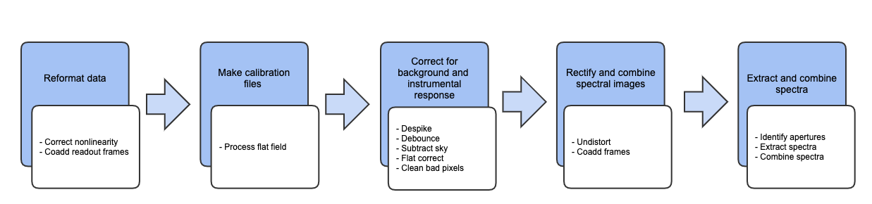
Fig. 1 Processing steps for EXES data.

Reduction algorithms

The following subsections detail each of the data reduction pipeline steps:

• Correct nonlinearity and coadd readout frames

• Process flat field

• Correct outliers (despike)

• Correct optical shifts (debounce)

• Subtract sky

• Flat correct

• Clean bad pixels

• Rectify spectral orders (undistort)

• Coadd frames

• Identify apertures

• Extract spectra

• Combine multiple spectra

Correct nonlinearity and coadd readout frames

Raw EXES data is stored in FITS image files, as a 3D data cube in which each plane corresponds to a digitized readout of the array. Readouts can be destructive or non-destructive. The readout method can vary for EXES, so the pattern of readout actions used for a particular observation is recorded in the OTPAT header keyword. The value for OTPAT is a combination of the letters S, T, N, D, and C, each with a digit afterwards. The letters have the following meaning:

• S = spin (no reset, no digitization). This action effectively increases the integration time.

• T = trash (reset, no digitization). This action resets the array without storing the previous value.

• N = non-destructive read (no reset, but digitized). This action stores the current value of the array.

• D = destructive read (reset and digitization). This action stores the current value, and resets the array.

• C = coadd (reset and digitization). This action coadds previous reads in hardware and resets the array.

The digit after each letter gives the number of times the action was taken, minus one. For example: S0 is one spin, N3 is four non-destructive reads.

The pattern listed in the OTPAT can then be repeated any number of times (\(n_{pat}\)), so that the final number of frames in the raw file is \(n_{pat} (n_{nd} + n_d)\), where \(n_{nd}\) is the number of nondestructive reads and \(n_d\) is the number of destructive reads per pattern.

Since near-infrared detectors do not have completely linear responses to incoming flux, each frame in the raw file may optionally be corrected for nonlinearity before proceeding. The nonlinearity coefficients for EXES were determined by taking a series of nondestructive flat exposures, followed by a single destructive read. Each readout was subtracted from a bias frame, then the resulting counts in each pixel were fit with a polynomial. The linearity correction algorithm reads in these polynomial coefficients from a 3D array and uses them to calculate a correction factor for each pixel in each raw readout. Pixels with counts below the bias level, or above the maximum value used to calculate the nonlinearity coefficients at that pixel, have no correction applied.

After linearity correction, in order to create a usable estimate of the input flux, the non-destructive and destructive reads must be combined in a way that maximizes the signal-to-noise. The EXES pipeline currently has support for combining frames taken with the patterns listed in the following subsections. Equations for the net signal and the associated variance come from Vacca et. al., 2004 (see Other Resources). After this initial calculation of the variance for each image pixel, the variance plane is propagated along with the image through all pipeline steps.

After the frames for each pattern are combined according to the algorithms below, the pipeline checks whether multiple patterns were taken at the same nod position. This is recorded in the header keyword NINT. If NINT is greater than 1, then NINT coadded patterns are averaged together before proceeding. Optionally, one or more of the initial patterns may be discarded before averaging.

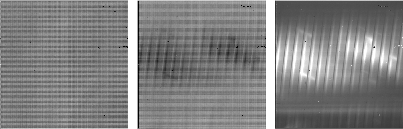
Fig. 2 Sample raw frames in nod-off-slit, High-Medium configuration: a pedestal image (left), a final destructive read (middle), and the Fowler coadd (right). The bright spectrum is visible as a dark line in the final raw readout and a bright line in the coadd.

All destructive mode

In this mode, each frame is a destructive read. There may be spins in between reads to increase integration time, but there are no non-destructive reads. In this case, the flux is simply the read signal (s), minus a standard bias frame (b) stored on disk, subtracted from a zero value (z), corresponding to a dark current, and divided by the integration time (\(\Delta t\)) and the pre-amp gain factor (\(g_p\)):

\[I_{net} = z - \frac{(s - b)}{\Delta t\ g_p}.\]

The dark current is typically zero for EXES.

The variance associated with this readout mode is the Poisson noise (first term) plus the readout noise (second term):

\[V = \frac{I_{net}}{g\ \Delta t} + \frac{{\sigma_{read}}^{2}}{g^2\ {\Delta t}^{2}},\]

where \(\sigma_{read}\) is the read noise, and g is the gain factor (to convert from ADU to electrons).

This readout mode may optionally be used for any readout pattern, ignoring the non-destructive reads and using the final destructive read only.

Fowler mode

In this mode, a number of non-destructive reads are taken at the beginning of the integration, the array integrates for a while, then a number of non-destructive reads and a single destructive read are taken at the end of the integration. The initial reads are averaged together to estimate the “pedestal” level; the final reads are averaged together to estimate the total signal. The pedestal is then subtracted from the total signal to get the net signal. We then subtract the negative signal from a zero value (z) and divide by the pre-amp gain factor (\(g_p\)) and the integration time (\(\Delta t\), the time between the first pedestal read and the first signal read). The net flux is then:

\[I_{net} = z - \frac{1}{n_r\ \Delta t\ g_p} \left( \sum_{i=1}^{n_r} s_i - \sum_{i=1}^{n_r}p_i \right).\]

We assume that the number of reads (\(n_r\)) is the same for the pedestal and the signal.

The variance associated with this readout mode is:

\[V = \frac{I_{net}}{g\ \Delta t}\left( 1 - \frac{\delta t \left( {n_r}^{2} - 1 \right)}{3\ \Delta t\ n_r} \right) + \frac{2\ {\sigma_{read}}^2}{g^2\ {\Delta t}^2\ n_r}.\]

Here, \(\delta t\) is the frame time, \(\sigma_{read}\) is the read noise, and g is the gain factor to convert from ADU to electrons.

Sample OTPAT values for Fowler mode look like this:

• N0 D0: a single non-destructive/destructive pair. This is the minimal Fowler case: the first read is the pedestal, the second read is the signal. There are 2 frames per pattern.

• N3 S15 N2 D0: a Fowler 4 set. This set comprises 4 non-destructive reads, 16 spins to increase the integration time, 3 non-destructive reads, and a destructive read. There are 8 frames per pattern.

Sample-up-the-ramp mode

In this mode, non-destructive reads are taken at even intervals throughout the integration. The count values for all reads are fit with a straight line; the slope of this line gives the net flux. As with the other modes, we then subtract from the zero value and divide by the pre-amp gain and the integration time. The net flux for the evenly-sampled case is calculated as:

\[I_{net} = z - \frac{12}{n_r\ \left( n_r + 1 \right) \Delta t\ g_p} \left( \sum_{i = 1}^{n_r} s_{i}\left\lbrack i - \frac{n_{r} + 1}{2} \right\rbrack \right),\]

where \(n_r\) is the total number of reads (non-destructive and destructive).

The variance associated with this readout mode is:

\[V = \frac{6\ I_{net} \left( {n_r}^2 + 1 \right)}{5\ g\ \Delta t\ n_r\ \left( n_r + 1 \right)} + \frac{12\ {\sigma_{read}}^{2} \left( n_r - 1 \right)}{g^2\ {\Delta t}^2\ n_r\ \left( n_r + 1 \right)}.\]

Sample OTPAT values for sample-up-the-ramp mode look like this:

• N0 S3 N0 S3 N0 S3 D0: Sample-up-the-ramp with 4 spins in between each non-destructive read, ending with a destructive read. There are 4 frames per pattern.

Coadding

If the OT pattern contains a coadd (C), it is treated as a destructive read for which the appropriate combination has already been done. That is, if the pattern indicates Fowler mode, for example, the intensity is simply calculated as for a destructive read:

\[I_{net} = z - \frac{s}{\Delta t\ g_p},\]

but the variance is calculated from the net intensity as for the Fowler mode, above.

Process flat field

Each EXES reduction requires a flat observation taken in the same mode as the science data. The instrument configuration (eg. HIGH_MED or MEDIUM), central wavenumber, slit height, slit width, and grating angle must all match. This flat observation is used to correct for spectral and spatial instrumental gain variations, and to calibrate the source intensity of the science observation.

The flat observation consists of an observation of a blackbody in EXES’s calibration box (black) and a dark frame (dark). If the blackbody’s temperature is known, then dividing the sky-subtracted science frame by black-dark, normalized by the blackbody function, gives a calibrated intensity as follows (Lacy et. al., 2002, see Other Resources).

\[ \begin{align}\begin{aligned}S_{\nu}(black-dark) &= B_{\nu}(T_{black})\ R_{\nu}\\S_{\nu}(obj-sky) &\approx I_{\nu}(obj)\ R_{\nu}\\I_{\nu}(obj) &\approx S_{\nu}(obj-sky)\ \frac{B_{\nu}(T_{black})}{S_{\nu}(black-dark)}\end{aligned}\end{align} \]

where \(S_{\nu}\) is the measured signal, \(B_{\nu}(T)\) is the blackbody function at temperature T, and \(R_{\nu}\) is the instrumental responsivity. The master flat frame produced by the EXES pipeline, therefore, is the blackbody function calculated at the temperature recorded in the flat frame’s header (BB_TEMP) and the central wavenumber for the observation (WAVENO0), divided by black-dark (Fig. 3). [1]

[1]

The flat value as derived is an approximation to the calibration function for all data in the spectrum: the true value depends slightly on the wavenumber value for each pixel in the spectrum. In pipeline version 3.0.0 and later, a correction for this wavenumber dependence is applied directly to the 2D spectral data, immediately following the undistort pipeline step.

In all instrument configurations, the black frame is also used to determine an illumination mask that defines the good pixels for extraction. In the cross-dispersed modes, the black frame is further used to determine the edges of the orders for extraction and to check the optical distortion parameters. The pipeline cleans and undistorts the black frame, takes its derivative, then performs a 2D FFT of the resulting image to determine the spacing and orientation of the orders on the array. In particular, the value of \(k_{rot}\), the angle of the order rotation, is adjusted automatically at this step: it is calculated from the characteristics of the FFT, then used to recompute the undistortion of the black frame, and redo the FFT, until the value of \(k_{rot}\) converges, or 5 iterations are reached. This process must be closely monitored: if the black frame has insufficient signal, or the optical parameters used to calculate the distortion correction are insufficiently accurate, the spacing and rotation angle may be wrongly calculated at this step. These values can be manually overridden in parameters for the pipeline if necessary.

The distortion parameters and order definitions, as determined from the black frame, are written to the header of the master flat, to be used in later reduction steps.

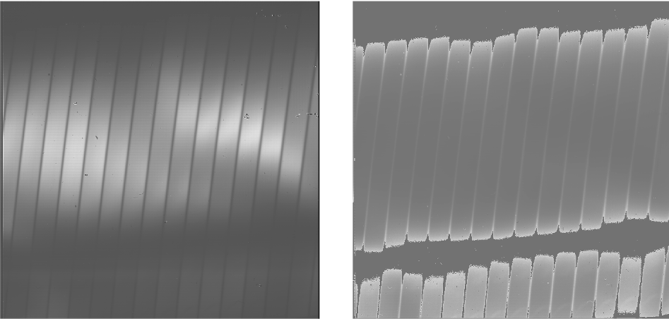
Fig. 3 Sample flat in High-Medium configuration. The left image is the black frame; the right image is the final processed flat frame. Unilluminated regions are set to zero in the final frame.

Despike

After coadding the raw frames to make A and B nod frames, the pipeline attempts to identify and correct spikes (outlier data points) in the individual images. All A frames are compared, and any pixels with values greater than a threshold number of standard deviations from the mean value across the other frames are replaced with that mean value. B frames are similarly compared with each other. The threshold for identifying spikes is a tunable parameter; the default value is 20 sigma. Also in the despike step, frames with significantly different overall background levels (“trashed” frames) may be identified automatically and removed from subsequent reduction. It is common, for example, for the first frame to look significantly different from the rest of the frames. In this case, leaving out this frame may improve the signal-to-noise of the final result.

Optionally, all input files may be combined at the despike step, prior to performing the outlier analysis. If the background levels do not differ significantly from one file to the next, this option can help perform better despiking on short or truncated observations.

Debounce

After despiking, there is an optional step called debouncing, which may help alleviate the effects of small optics shifts (“bounces”) between the nod beams. If there is a slight mismatch in the order placement on the array, it can lead to poor background subtraction when the nods are subtracted. In the debouncing algorithm, each nod pair is undistorted, then the B nod is shifted slightly in the spatial direction and differenced with the A nod. The shift direction that results in a minimum squared difference (summed over the spectral direction) is used as the bounce direction. The amplitude of the shift is controlled by the bounce parameter, which should be set to a number whose absolute value is between 0 and 1 (typically 0.1). If the bounce parameter is set to a positive number, only the above shift (the first-derivative bounce) will be corrected. If the bounce parameter is set to a negative value (e.g. -0.1), the debouncing algorithm will also attempt to fix the second-derivative bounce by smoothing the A or B nod slightly; the amount of smoothing is also controlled by the absolute value of the bounce parameter. Note that if the observed source is too near the edge of the order, it may confuse the debouncing algorithm; in this case, it is usually best to turn debouncing off (i.e. set the bounce parameter to 0). The default is not to use the debounce algorithm.

Subtract sky

In either nod-on-slit or nod-off-slit mode, each B nod is subtracted from each adjacent A nod (Fig. 4). This step usually removes most of the background emission from the image, but if there were changes in the sky level between the two nod frames, there may still be some residual sky signal. For the nod-off-slit mode, this residual signal can be estimated and corrected for before subtracting the nods, by subtracting a weighted fraction of the B data from the A data. The weighting is chosen to minimize the squared difference between the A and B nods. For the nod-on-slit mode, the mean background at each wavelength may be subtracted after nod subtraction and distortion correction, so that the wavelengths align with columns in the image. The pipeline performs this step immediately before coadding, if desired.

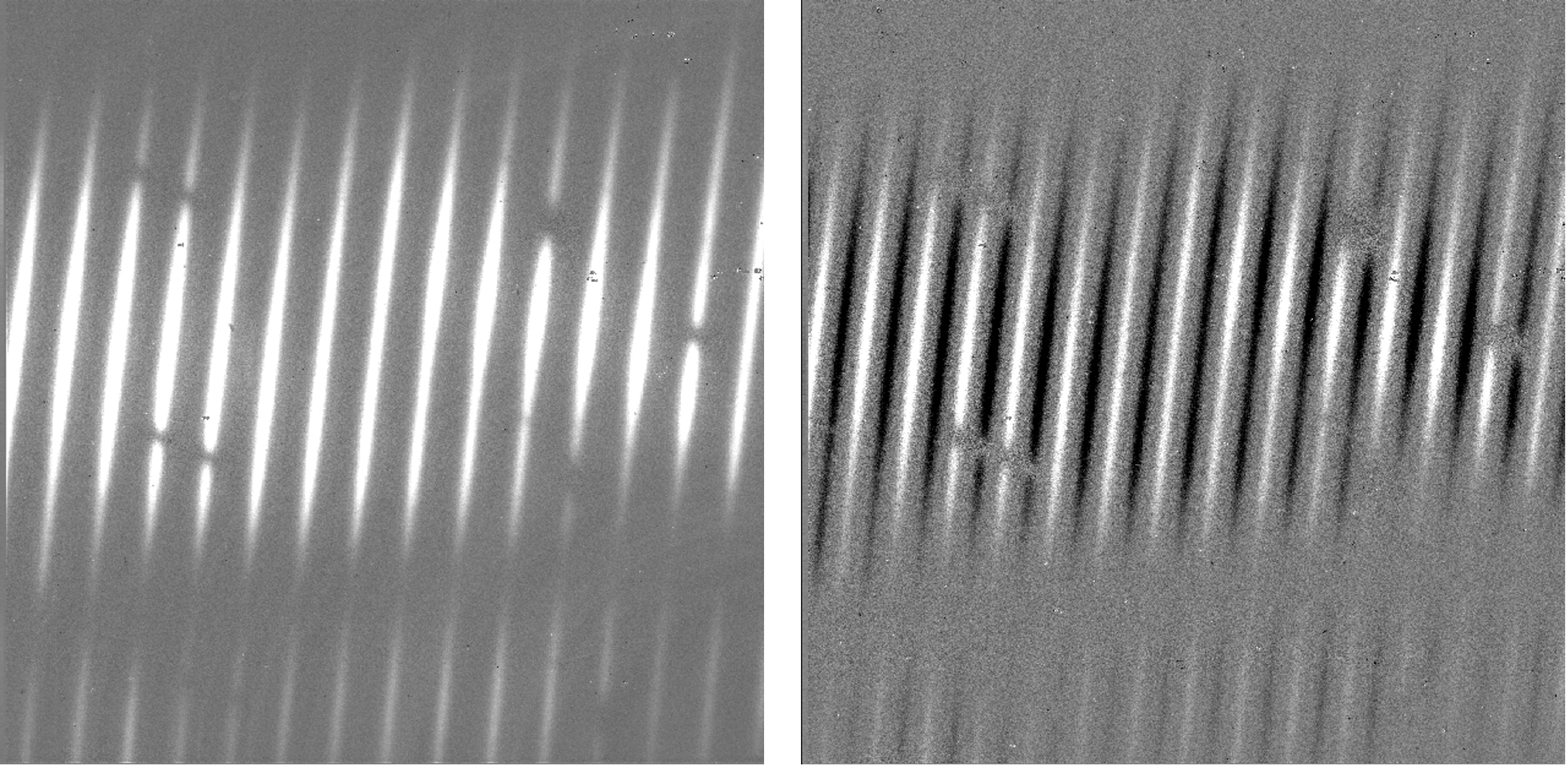
Fig. 4 Background subtracted frames in nod-off-slit (left) and nod-on-slit (right), in High-Medium configuration.

For the mapping mode, each of the steps across the source is treated as an A frame. The three sky frames taken at the end of the map are averaged together and this average is subtracted from each A frame (Fig. 5). This mode is usually used for extended sources that fill the entire slit, in which case there is no way to estimate or correct for any residual background remaining after sky subtraction. The three sky frames at the end of the map can be part of the map (without science target signal) or dedicated sky positions away from the source.

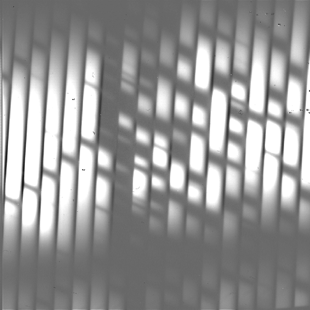
Fig. 5 Background subtracted image in High-Medium configuration with map mode. The extended source fills the entire slit.

Flat correct

After background subtraction, each science frame is multiplied by the processed flat calibration frame, described above. This has the effect of both correcting the science frame for instrumental response and calibrating it to intensity units.

Clean bad pixels

In this step, bad pixels are identified and corrected. Bad pixels may first be identified in a bad pixel mask, provided by the instrument team. In this FITS image, pixels that are known to be bad are marked with a value of 0; good pixels are marked with a value of 1. Alternately, bad pixels may be identified from their noise characteristics: if the error associated with a pixel is greater than a threshold value (by default: 20) times the mean error for the frame, then it is marked as a bad pixel. Unlike the despike algorithm, which identifies outliers by comparing separate frames, outliers in this algorithm are identified by comparing the values within a single frame.

Bad pixels may be corrected by using neighboring good values to linearly interpolate over the bad ones. The search for good pixels checks first in the y-direction, then in the x-direction. If good pixels cannot be identified within a 10-pixel radius, then the bad pixel will not be corrected. Alternately, bad pixels may be flagged for later handling by setting their values to NaN. In this case, bad pixels are ignored in later coaddition and extraction steps.

Note that bad pixels may also be fixed or ignored in the spectral extraction process, so it is not critical to correct all bad pixels at this stage.

Undistort

Next, the pipeline corrects the image for optical distortion, resampling the image onto a regular grid of spatial and spectral elements. The EXES distortion correction uses knowledge of the optical design of the instrument, as well as data recorded in the header of the observation, to calculate and correct for the optical distortion in each observation.

The optical parameters used to calculate the distortion correction are listed in the table below. Most of these parameters should not change, or should change rarely, so they have default values listed in configuration tables available to the pipeline (the .dat files listed below). Values in the tortparm.dat configuration table tend to change over time, as the instrument is adjusted, so their defaults vary by date. Some of the distortion parameters must come from the headers and do not have default values. One parameter is tuned at run-time (krot), and one must be manually optimized by the user (waveno0).

Table 1 Optical distortion parameters.

Parameter	Default value	Source	Comment
hrfl	(varies by date)	tortparm.dat	High resolution chamber focal length
xdfl	(varies by date)	tortparm.dat	Assumed cross- dispersed focal length
slitrot	(varies by date)	tortparm.dat	Slit rotation
detrot	(varies by date)	tortparm.dat	Detector rotation
hrr	(varies by date)	tortparm.dat	R number for echelon grating
brl	0.00	tortparm.dat	Barrel distortion parameter
x0brl	0.00	tortparm.dat	X-coordinate for the center of the barrel distortion
y0brl	0.00	tortparm.dat	Y-coordinate for the center of the barrel distortion
hrg	-0.015	headerdef.dat	Gamma (out of plane) angle for the echelon grating (radians)
xdg	0.033	headerdef.dat	Gamma angle for cross- dispersion grating (radians)
xdlrdgr	0.001328	headerdef.dat	Low resolution groove spacing (cm)
xdmrdgr	0.003151	headerdef.dat	Medium resolution groove spacing (cm)
pixelwd	0.0025	headerdef.dat	Pixel width
waveno0	(none)	Header keyword WAVENO0	Planned central wavenumber
echelle	(none)	Header keyword ECHELLE	Echelle grating angle (deg)
krot	(varies by date)	tortparm.dat / Optimized at run-time	Rotation between chambers

Several of these parameters are then combined or recalculated before being used in the distortion correction. The cross-dispersed R number (xdr) is calculated from the groove spacing (xdlrdgr or xdmrdgr), the grating angle (echelle), and the central wavenumber (waveno0). The expected order spacing for cross-dispersed modes is calculated from the cross-dispersed R number (xdr), the cross-dispersed focal length (xdfl), the pixel width (pixelwd), and the echelon gamma angle (hrg). The order spacing and the rotation angle (krot) are optimized for cross-dispersed modes when the calibration frame is processed, as described above.

The distortion correction equations calculate undistorted coordinates by correcting for the following effects for the cross-dispersed modes:

• slit skewing within orders due to the echelon “smile” (hrg, hrr, slitrot)

• nonlinearity of the echelon spectrum (hrr, pixelwd, hrfl)

• skewing by spectrum rotation on the detector due to the angle between the chambers, and the cross-dispersion smile (xdg, xdr, krot, pixelwd, xdfl, hrfl, hrr)

• nonlinearity of the cross-dispersion spectrum (xdr, pixelwd, xdfl)

• barrel distortion (brl, x0brl, y0brl)

For the long-slit modes, the distortion correction accounts for:

• skewing by the cross-dispersion smile (xdg, xdr, slitrot, pixelwd, xdfl)

• nonlinearity of the cross-dispersion spectrum (xdr, pixelwd, xdfl)

• barrel distortion (brl, x0brl, y0brl)

When the undistorted coordinates have been calculated, the 2D science image is interpolated from raw (x,y) pixel coordinates onto these coordinates. By default, a cubic interpolation is used that closely approximates a sinc interpolation function; bilinear interpolation is also available.

After distortion correction, the spatial and spectral elements should be aligned with the columns and rows of the image (Fig. 6). For both long-slit and cross-dispersed modes, the x-axis is the dispersion axis and the y-axis is the spatial axis. Values outside the illuminated areas for each spectral order are set to NaN.

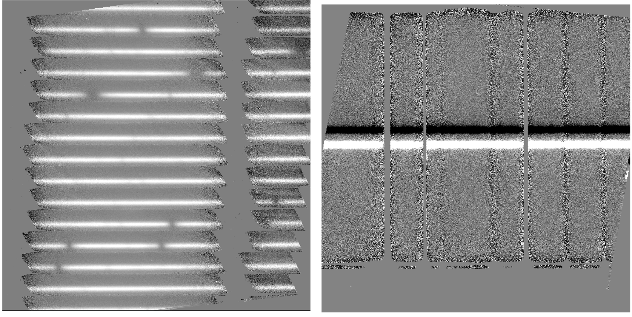
Fig. 6 Undistorted images in High-Medium configuration (left) and Medium configuration (right).

Coadd frames

The final step in the image processing prior to spectral extraction is coadding of the background-subtracted, undistorted frames (Fig. 7). If desired, coaddition can be skipped, and individual spectra can be extracted from each frame, to be combined later. For faint sources, however, coaddition of the 2D image is recommended, for more accurate extraction.

Prior to coadding, the spectra can be shifted in the spatial direction to account for slight shifts in the position of the object in the slit between nod pairs. The shift is calculated by creating a template of the spectrum from all frames, averaged in the spectral direction, and cross-correlating each frame with the template.

By default, the pipeline weights all input frames by their correlation with this spectral template, so that if a frame is unusually noisy, or missed a nod, or had some other error, it will not contribute significantly to the coadded frame. However, it is possible to force the pipeline to use an unweighted coadd, if desired, or to explicitly identify frames for exclusion from the coadd.

The pipeline typically only coadds frames within a single file. Optionally, it may instead coadd frames from all files. This action is performed as an robust mean across all input frames, with or without weighting by the associated error image. In cases where the target has not moved across the array between input files, this option may help increase signal-to-noise prior to extraction.

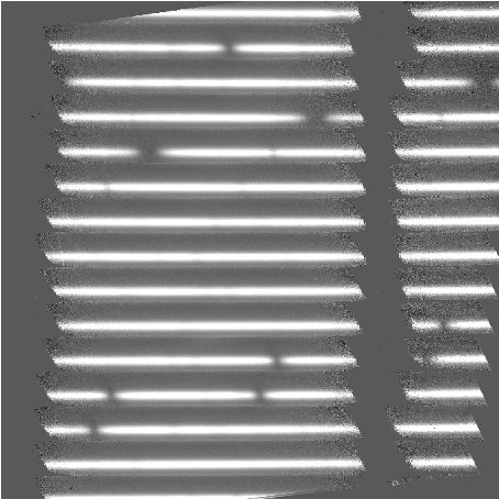
Fig. 7 Coadded image in High-Medium configuration.

Identify apertures

In order to aid in spectral extraction, the pipeline constructs a smoothed model of the relative intensity of the target spectrum at each spatial position, for each wavelength. This spatial profile is used to compute the weights in optimal extraction or to fix bad pixels in standard extraction (see next section). Also, the pipeline uses the median profile, collapsed along the wavelength axis, to define the extraction parameters.

To construct the spatial profile, the pipeline first subtracts the median signal from each column in the rectified spectral image to remove the residual background. The intensity in this image in column i and row j is given by

\[O_{ij} = f_{i}P_{ij}\]

where \(f_i\) is the total intensity of the spectrum at wavelength i, and \(P_{ij}\) is the spatial profile at column i and row j. To get the spatial profile \(P_{ij}\), we must approximate the intensity \(f_i\). To do so, the pipeline computes a median over the wavelength dimension (columns) of the order image to get a first-order approximation of the median spatial profile at each row \(P_j\). Assuming that

\[O_{ij} \approx c_{i}P_{j},\]

the pipeline uses a linear least-squares algorithm to fit \(P_j\) to \(O_{ij}\) and thereby determine the coefficients \(c_i\). These coefficients are then used as the first-order approximation to \(f_i\): the resampled order image \(O_{ij}\) is divided by \(f_i\) to derive \(P_{ij}\). The pipeline then fits a low-order polynomial along the columns at each spatial point s in order to smooth the profile and thereby increase its signal-to-noise. The coefficients of these fits can then be used to determine the value of \(P_{ij}\) at any column i and spatial point j (see Fig. 8, left). The median of \(P_{ij}\) along the wavelength axis generates the median spatial profile, \(P_j\) (see Fig. 8, right).

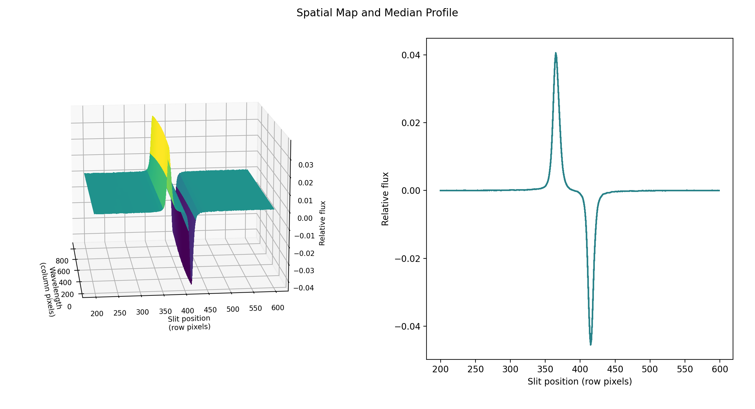
Fig. 8 Spatial model and median spatial profile, for the Medium configuration image in Fig. 6. The spatial model image here is rotated for comparison with the profile plot: the y-axis is along the bottom of the surface plot; the x-axis is along the left.

The pipeline then uses the median spatial profile to identify extraction apertures for the source. The aperture centers can be identified automatically by iteratively finding local maxima in the absolute value of the spatial profile, or can be specified directly by the user. By default, a single aperture is expected and defined for nod-off-slit mode; two apertures are expected for nod-along-slit mode.

Besides the aperture centers, the pipeline also specifies a PSF radius, corresponding to the distance from the center at which the flux from the source falls to zero. By default, this value is automatically determined from the width of a Gaussian fit to the peak in the median spatial profile, as

\[R_{psf} = 2.15 \cdot \text{FWHM}.\]

For optimal extraction, the pipeline also identifies a smaller aperture radius, to be used as the integration region:

\[R_{ap} = 0.7 \cdot \text{FWHM}.\]

This value should give close to optimal signal-to-noise for a Moffat or Gaussian profile. The pipeline also attempts to specify background regions outside of any extraction apertures, for fitting and removing the residual sky signal. All aperture parameters may be optionally overridden by the pipeline user.

Extract spectra

The spectral extraction algorithms used by the pipeline offer two different extraction methods, depending on the nature of the target source. For point sources, the pipeline uses an optimal extraction algorithm, described at length in the Spextool paper (see the Other Resources section, below, for a reference). For extended sources, the pipeline uses a standard summing extraction.

In either method, before extracting a spectrum, the pipeline first uses any identified background regions to find the residual sky background level. For each column in the 2D image, it fits a low-order polynomial to the values in the specified regions, as a function of slit position. This polynomial determines the wavelength-dependent sky level (\(B_{ij}\)) to be subtracted from the spectrum (\(D_{ij}\)).

Standard extraction

The standard extraction method uses values from the spatial profile image (\(P_{ij}\)) to replace bad pixels and outliers, then sums the flux from all pixels contained within the PSF radius. The flux at column i is then:

\[f_{i,\text{sum}} = \sum_{j=j_1}^{j_2}(D_{ij} - B_{ij})\]

where \(j_1\) and \(j_2\) are the upper and lower limits of the extraction aperture (in pixels):

\[ \begin{align}\begin{aligned}j_1 &= t - R_{PSF}\\j_2 &= t + R_{PSF}\end{aligned}\end{align} \]

given the aperture center (t). This extraction method is the only algorithm available for extended sources.

Optimal extraction

Point sources may occasionally benefit from using standard extraction, but optimal extraction generally produces higher signal-to-noise ratios for these targets. This method works by weighting each pixel in the extraction aperture by how much of the target’s flux it contains. The pipeline first normalizes the spatial profile by the sum of the spatial profile within the PSF radius defined by the user:

\[P_{ij}^{'} = P_{ij} \Big/ \sum_{j=j_1}^{j_2}P_{ij}.\]

\(P_{ij}^{'}\) now represents the fraction of the total flux from the target that is contained within pixel (i,j), so that \((D_{ij} - B_{ij}) / P_{ij}^{'}\) is a set of j independent estimates of the total flux at column i. The pipeline does a weighted average of these estimates, where the weight depends on the pixel’s variance and the normalized profile value. Then, the flux at column i is:

\[f_{i,\text{opt}} = \frac{\sum_{j=j_3}^{j_4}{M_{ij}P_{ij}^{'}(D_{ij} - B_{ij}) \big/ (V_{D_{ij}} + V_{B_{ij}})}}{\sum_{j=j_3}^{j_4}{M_{ij}{P_{ij}^{'}}^{2} \big/ (V_{D_{ij}} + V_{B_{ij}})}}\]

where \(M_{ij}\) is a bad pixel mask and \(j_3\) and \(j_4\) are the upper and lower limits given by the aperture radius:

\[ \begin{align}\begin{aligned}j_3 &= t - R_{ap}\\j_4 &= t + R_{ap}\end{aligned}\end{align} \]

Note that bad pixels are simply ignored, and outliers will have little effect on the average because of the weighting scheme.

The variance for the standard spectroscopic extraction is a simple sum of the variances in each pixel within the aperture. For the optimal extraction algorithm, the variance on the \(i^{th}\) pixel in the extracted spectrum is calculated as:

\[V_{i} = \sum_{j=j_3}^{j_4} \frac{M_{ij}}{{P_{ij}^{'}}^2 V_{ij}}\]

where \(P_{ij}^{'}\) is the scaled spatial profile, \(M_{ij}\) is a bad pixel mask, \(V_{ij}\) is the variance at each background-subtracted pixel, and the sum is over all spatial pixels \(j\) within the aperture radius. The error spectrum for 1D spectra is the square root of the variance.

Wavelength calibration

Wavelength calibration for EXES is calculated from the grating equation, using the optical parameters and central wavenumber for the observation. It is stored as a calibration map identifying the wavenumber for each column in each spectral order.

The wavelength calibration is expected to be good to within one pixel of dispersion, if the central wavenumber is accurate. To refine the wavelength solution, the pipeline allows the user to identify a single spectral feature in the extracted spectrum. Using this feature, the central wavenumber is recalculated and the calibration is adjusted to match. However, the distortion correction also depends on the central wavenumber, so if the recalculated value is significantly different from the assumed value, the reduction should be repeated with the new value to ensure an accurate distortion correction and dispersion solution.

Combine multiple spectra

The final pipeline step is the combination of multiple spectra of the same source, from separate observations, apertures, and orders. For all configurations, the individual extracted 1D spectra for each order are combined with a robust weighted mean, by default.

For cross-dispersed configurations, the pipeline performs an automatic merge of the spectra from all orders. This algorithm uses the signal-to-noise ratio in overlapping regions to determine which pixels to exclude, and performs a weighted mean of any remaining overlapping regions. Artifacts near the edges of orders may optionally be manually trimmed before the merge.

Other Resources

For more information on the reduction algorithms used in the EXES package, adapted from the TEXES pipeline, see the TEXES paper:

TEXES: A Sensitive High-Resolution Grating Spectrograph for the Mid-Infrared, J.H. Lacy, M.J. Richter, T.K. Greathouse, D.T. Jaffe and Q. Zhu (2002, PASP 114, 153)

For more information on the reduction algorithms used in FSpextool, see the Spextool papers:

Spextool: A Spectral Extraction Package for SpeX, a 0.8-5.5 Micron Cross-Dispersed Spectrograph, Michael C. Cushing, William D. Vacca and John T. Rayner (2004, PASP 116, 362).

A Method of Correcting Near-Infrared Spectra for Telluric Absorption, William D. Vacca, Michael C. Cushing and John T. Rayner(2003, PASP 115, 389).

Nonlinearity Corrections and Statistical Uncertainties Associated with Near-Infrared Arrays, William D. Vacca, Michael C. Cushing and John T. Rayner (2004, PASP 116, 352).

Flux calibration

EXES spectra are calibrated to physical intensity units (\(erg/s/cm^2/sr/cm^{-1}\)) when they are multiplied by the blackbody-normalized calibration frame. This process does not account for residual atmospheric effects. These may be corrected by dividing by a telluric standard spectrum, or a model of the atmosphere.

Following the coaddition of 2D spectral images from each nod pair, a conversion factor is applied to convert the units to integrated flux units of Jy per spatial pixel for 2D images. Extraction performed on these images sums over spatial pixels, resulting in units of Jy for all 1D spectra. To derive a surface brightness value from 1D spectra, such as Jy/arcsec, refer to the aperture width in the FITS header (PSFRADn, for order n = 01, 02, 03…).

Please note that the absolute flux calibration for EXES targets may require additional corrections for slit loss, instrument response, poorly determined background levels, or other systematic effects.

Data products

Filenames

EXES output files are named according to the convention:

FILENAME = F[flight]_EX_SPE_AOR-ID_SPECTEL1SPECTEL2_type_FN1[-FN2][_SN].fits

where flight is the SOFIA flight number, EX is the instrument identifier, SPE specifies that it is a spectral file, AOR-ID is the AOR identifier for the observation, SPECTEL1SPECTEL2 are the keywords specifying the spectral elements used, type is the three-letter identifier for the product type (listed in the table below), and FN1 is the file number corresponding to the input file. FN1-FN2 is used if there are multiple input files for a single output file, where FN1 is the file number of the first input file and FN2 is the file number of the last input file. If the output file corresponds to a single frame of the input file, there may also be a trailing serial number (SN) that identifies the input frame associated with the output file.

Pipeline Products

The following table lists all intermediate products generated by the pipeline for EXES spectral modes, in the order in which they are produced. [2] The product type is stored in the FITS headers under the keyword PRODTYPE. By default, the readouts_coadded, flat, undistorted, coadded, spectra, spectra_1d, coadded_spectrum, combined_spectrum_1d, orders_merged, and orders_merged_1d products are saved.

For calibration purposes, it is often useful to set pipeline parameters to skip nod subtraction and extract a sky spectrum rather than a science spectrum. Data products reduced in this mode have separate product types, with ‘sky_’ prepended to the standard product name, and file codes that begin with the letter ‘S’.

For most observation modes, the pipeline additionally produces an image in PNG format, intended to provide a quick-look preview of the data contained in the final product. These auxiliary products may be distributed to observers separately from the FITS file products.

[2]

Earlier versions of this pipeline (before v3.0.0) produced different sets of default products. Refer to earlier revisions of this manual for complete information.

Table 2 Intermediate and final data products for EXES reductions

Step	Data type	PRODTYPE	PROCSTAT	Code	Saved	Extensions
Coadd Readouts	2D spectral image	readouts_ coadded	LEVEL_2	RDC	Y	FLUX, ERROR, MASK
Make Flat	2D spectral image	flat_ appended	LEVEL_2	FTA	N	FLUX, ERROR, MASK, FLAT, FLAT_ERROR, FLAT_ILLUMINATION
Make Flat	2D spectral flat	flat	LEVEL_2	FLT	Y	FLAT, FLAT_ERROR, TORT_FLAT, TORT_FLAT_ERROR, ILLUMINATION, WAVECAL, SPATCAL, ORDER_MASK
Despike	2D spectral image	despiked	LEVEL_2	DSP	N	FLUX, ERROR, MASK, FLAT, FLAT_ERROR, FLAT_ILLUMINATION
Debounce	2D spectral image	debounced	LEVEL_2	DBC	N	FLUX, ERROR, MASK, FLAT, FLAT_ERROR, FLAT_ILLUMINATION
Subtract Nods	2D spectral image	nods_ subtracted or sky_nods_ subtracted	LEVEL_2	NSB or SNS	N	FLUX, ERROR, MASK, FLAT, FLAT_ERROR, FLAT_ILLUMINATION
Flat Correct	2D spectral image	flat_ corrected or sky_flat_ corrected	LEVEL_2	FTD or SFT	N	FLUX, ERROR, MASK, FLAT, FLAT_ERROR, FLAT_ILLUMINATION
Clean Bad Pixels	2D spectral image	cleaned or sky_cleaned	LEVEL_2	CLN or SCN	N	FLUX, ERROR, MASK, FLAT, FLAT_ERROR, FLAT_ILLUMINATION
Undistort	2D spectral image	undistorted or sky_ undistorted	LEVEL_2	UND or SUN	Y	FLUX, ERROR, MASK, FLAT, FLAT_ERROR, FLAT_ILLUMINATION, WAVECAL, SPATCAL, ORDER_MASK
Correct Calibration	2D spectral image	calibration_ corrected or sky_ calibration_ corrected	LEVEL_2	CCR or SCR	N	FLUX, ERROR, MASK, FLAT, FLAT_ERROR, FLAT_ILLUMINATION, WAVECAL, SPATCAL, ORDER_MASK
Coadd Pairs	2D spectral image	coadded or sky_coadded	LEVEL_2	COA or SCO	Y	FLUX, ERROR, MASK, FLAT, FLAT_ERROR, FLAT_ILLUMINATION, WAVECAL, SPATCAL, ORDER_MASK
Convert Units	2D spectral image	calibrated or sky_calibrated	LEVEL_2	CAL or SCL	Y	FLUX, ERROR, MASK, FLAT, FLAT_ERROR, FLAT_ILLUMINATION, WAVECAL, SPATCAL, ORDER_MASK
Make Profiles	2D spectral image	rectified_ image or sky_ rectified_ image	LEVEL_2	RIM or SRM	N	FLUX, ERROR, MASK, FLAT, WAVECAL, SPATCAL, FLAT_ILLUMINATION, For each order n: FLUX_ORDER_n ERROR_ORDER_n FLAT_ORDER_n BADMASK_ORDER_n WAVEPOS_ORDER_n SLITPOS_ORDER_n SPATIAL_MAP_ORDER_n SPATIAL_PROFILE_ORDER_n
Locate Apertures	2D spectral image	apertures_ located or sky_ apertures_ located	LEVEL_2	LOC or SLC	N	FLUX, ERROR, MASK, FLAT, WAVECAL, SPATCAL, ORDER_MASK For each order n: FLUX_ORDER_n ERROR_ORDER_n FLAT_ORDER_n BADMASK_ORDER_n WAVEPOS_ORDER_n SLITPOS_ORDER_n SPATIAL_MAP_ORDER_n SPATIAL_PROFILE_ORDER_n
Set Apertures	2D spectral image	apertures_ set or sky_ apertures_ set	LEVEL_2	APS or SAP	N	FLUX, ERROR, MASK, FLAT, WAVECAL, SPATCAL, ORDER_MASK For each order n: FLUX_ORDER_n ERROR_ORDER_n FLAT_ORDER_n BADMASK_ORDER_n WAVEPOS_ORDER_n SLITPOS_ORDER_n SPATIAL_MAP_ORDER_n SPATIAL_PROFILE_ORDER_n APERTURE_MASK_ORDER_n
Subtract Background	2D spectral image	background_ subtracted or sky_ background_ subtracted	LEVEL_2	BGS or SBG	N	FLUX, ERROR, MASK, FLAT, WAVECAL, SPATCAL, ORDER_MASK For each order n: FLUX_ORDER_n ERROR_ORDER_n FLAT_ORDER_n BADMASK_ORDER_n WAVEPOS_ORDER_n SLITPOS_ORDER_n SPATIAL_MAP_ORDER_n SPATIAL_PROFILE_ORDER_n APERTURE_MASK_ORDER_n
Extract Spectra	2D spectral image; 1D spectrum	spectra or sky_ spectra	LEVEL_2	SPM or SSM	Y	FLUX, ERROR, MASK, FLAT, WAVECAL, SPATCAL, ORDER_MASK, TRANSMISSION For each order n: FLUX_ORDER_n ERROR_ORDER_n FLAT_ORDER_n BADMASK_ORDER_n WAVEPOS_ORDER_n SLITPOS_ORDER_n SPATIAL_MAP_ORDER_n SPATIAL_PROFILE_ORDER_n APERTURE_MASK_ORDER_n SPECTRAL_FLUX_ORDER_n SPECTRAL_ERROR_ORDER_n TRANSMISSION_ORDER_n RESPONSE_ORDER_n
Extract Spectra	1D spectrum	spectra_1d or sky_ spectra_1d	LEVEL_2	SPC or SSP	Y	FLUX
Combine Spectra	2D spectral image; 1D spectrum	coadded_ spectrum or sky_ coadded_ spectrum	LEVEL_2	COM or SCM	Y	FLUX, ERROR, TRANSMISSION For each order n: FLUX_ORDER_n ERROR_ORDER_n WAVEPOS_ORDER_n SPECTRAL_FLUX_ORDER_n SPECTRAL_ERROR_ORDER_n TRANSMISSION_ORDER_n RESPONSE_ORDER_n
Combine Spectra	1D spectrum	combined_ spectrum_1d or sky_ combined_ spectrum_1d	LEVEL_2	CMB or SCS	Y	FLUX
Refine Wavecal	2D spectral image; 1D spectrum	wavecal_ refined or sky_ wavecal_ refined	LEVEL_2	WRF or SWR	Y	FLUX, ERROR, TRANSMISSION For each order n: FLUX_ORDER_n ERROR_ORDER_n WAVEPOS_ORDER_n SPECTRAL_FLUX_ORDER_n SPECTRAL_ERROR_ORDER_n TRANSMISSION_ORDER_n RESPONSE_ORDER_n
Refine Wavecal	1D spectrum	wavecal_ refined_1d or sky_ wavecal_ refined_1d	LEVEL_2	WRS or SWS	Y	FLUX
Merge Orders	2D spectral image; 1D spectrum	orders_ merged or sky_orders_ merged	LEVEL_3	MRM or SMM	Y	FLUX, ERROR, WAVEPOS, SPECTRAL_FLUX, SPECTRAL_ERROR, TRANSMISSION, RESPONSE
Merge Orders	1D spectrum	orders_ merged_1d or sky_orders_ merged_1d	LEVEL_3	MRD or SMD	Y	FLUX

Data Format

All files produced by the pipeline are multi-extension FITS files (except for the spectra_1d, combined_spectrum_1d, and orders_merged_1d products: see below). [3] The flux image is stored in the primary header-data unit (HDU); its associated error image is stored in extension 1, with EXTNAME=ERROR.

In spectroscopic products, the SLITPOS and WAVEPOS extensions give the spatial (rows) and spectral (columns) coordinates, respectively, for rectified images for each order. These coordinates may also be derived from the WCS in the primary header. WAVEPOS also indicates the wavenumber coordinates for 1D extracted spectra.

Intermediate spectral products may contain SPATIAL_MAP and SPATIAL_PROFILE extensions. These contain the spatial map and median spatial profile, described in the Identify apertures section, above. They may also contain an APERTURE_MASK extension with the spectral aperture definitions, also described in the Identify apertures section.

Final spectral products contain SPECTRAL_FLUX and SPECTRAL_ERROR extensions: these are the extracted 1D spectrum and associated uncertainty. They also contain TRANSMISSION and RESPONSE extensions for reference, containing a model of the atmospheric transmission at the extracted wavenumber values and an extraction of the flat calibration data at the science aperture locations, respectively.

The spectra_1d, combined_spectrum_1d, and orders_merged_1d products are one-dimensional spectra, stored in Spextool format, as rows of data in the primary extension. If there were multiple orders in the intermediate spectra (e.g. the High-Medium configuration) or multiple apertures selected (e.g. for the nod-on-slit mode), then the spectrum for each aperture and order is stacked into a different plane.

For these spectra, the first row is the wavenumber (\(cm^{-1}\)), the second is the intensity (\(erg/s/cm^2/sr/cm^{-1}\)), the third is the error (\(erg/s/cm^2/sr/cm^{-1}\)), the fourth is the estimated fractional atmospheric transmission spectrum, and the fifth is a reference response spectrum (\(ct/(erg/s/cm^2/sr/cm^{-1})\)). These rows correspond directly to the WAVEPOS, SPECTRAL_FLUX, SPECTRAL_ERROR, TRANSMISSION, and RESPONSE extensions in the spectra, coadded_spectrum, or orders_merged products.

The final uncertainties in calibrated images and spectra contain only the estimated statistical uncertainties due to the noise in the image or the extracted spectrum. Any systematic uncertainties due to the reduction or calibration process are not recorded.

[3]

In earlier versions of this pipeline (prior to v3.0.0), all image products were 3D arrays of data, where the first half of the planes were the image frames and the second half of the planes were the variances associated with each pixel in each image frame. All spectral products were in the Spextool format described above.

Grouping LEVEL_1 data for processing

For EXES spectroscopy modes, there are three kinds of data: darks, flats, and sources. Flats and darks are required for all reductions, as they are used to calibrate the data, correct for instrumental response, and identify the edges of the slit. Dark frames should be taken near in time to the flat frame. Flat frames should have the same instrument configuration, slit height, slit width, and grating angle as the science observation. In order for separate science files to be grouped together, these same conditions apply, and they should additionally share a common target and be taken with the same nodding mode.

These requirements translate into a set of FITS header keywords that must match in order for a set of data to be usefully reduced together: see the table below for a listing of these keywords. All match requirements apply to science targets; flat exceptions are noted.

Note that data grouping must be carried out before the pipeline is run. The pipeline expects all inputs to be reduced together as a single data set.

Table 3 Grouping criteria

Keyword	Datatype	Match Criterion
INSTCFG	STR	Exact
SPECTEL1	STR	Exact
SPECTEL2	STR	Exact
SLIT	STR	Exact
ECHELLE	FLT	Exact
SDEG	FLT	Exact
WAVENO0	FLT	Exact
MISSN-ID	STR	Exact
ALTI_STA	FLT	+/- 500
ALTI_END	FLT	+/- 500
ZA_START	FLT	+/- 2.5
ZA_END	FLT	+/- 2.5
OBSTYPE	STR	Exact (unless flat)
OBJECT	STR	Exact (unless flat)
INSTMODE	STR	Exact (unless flat)
PLANID	STR	Exact (unless flat)
AOR-ID (optional)	STR	Exact (unless flat)

Configuration and execution

Installation

The EXES pipeline is written entirely in Python. The pipeline is platform independent and has been tested on Linux, Mac OS X, and Windows operating systems. Running the pipeline requires a minimum of 16GB RAM, or equivalent-sized swap file.

The pipeline is comprised of five modules within the sofia_redux package: sofia_redux.instruments.exes, sofia_redux.pipeline, sofia_redux.calibration, sofia_redux.spectroscopy, sofia_redux.toolkit, and sofia_redux.visualization. The exes module provides the data processing algorithms specific to EXES, with supporting libraries from the toolkit, calibration, spectroscopy, and visualization modules. The pipeline module provides interactive and batch interfaces to the pipeline algorithms.

External Requirements

To run the pipeline for any mode, Python 3.8 or higher is required, as well as the following packages: numpy, scipy, matplotlib, pandas, astropy, configobj, numba, bottleneck, joblib, and photutils. Some display functions for the graphical user interface (GUI) additionally require the PyQt5, pyds9, and regions packages. All required external packages are available to install via the pip or conda package managers. See the Anaconda environment file (environment.yml), or the pip requirements file (requirements.txt) distributed with sofia_redux for up-to-date version requirements.

Running the pipeline interactively also requires an installation of SAO DS9 for FITS image display. See http://ds9.si.edu/ for download and installation instructions. The ds9 executable must be available in the PATH environment variable for the pyds9 interface to be able to find and control it. Please note that pyds9 is not available on the Windows platform.

Source Code Installation

The source code for the EXES pipeline maintained by the SOFIA Data Processing Systems (DPS) team can be obtained directly from the DPS, or from the external GitHub repository. This repository contains all needed configuration files, auxiliary files, and Python code to run the pipeline on EXES data in any observation mode.

After obtaining the source code, install the package with the command:

python setup.py install

from the top-level directory.

Alternately, a development installation may be performed from inside the directory with the command:

pip install -e .

After installation, the top-level pipeline interface commands should be available in the PATH. Typing:

redux

from the command line should launch the GUI interface, and:

redux_pipe -h

should display a brief help message for the command line interface.

Configuration

For EXES algorithms, default parameter values are defined by the Redux object that interfaces to them. These values may be overridden manually for each step, while running in interactive mode. They may also be overridden by an input parameter file, in INI format, in either interactive or automatic mode. See Appendix A for an example of an input parameter file, which contains the current defaults for all parameters.

Input data

Redux takes as input raw EXES FITS data files, which are image cubes composed of 1024 x 1024 pixel image arrays. The number of frames per raw data cube depends on the readout mode used to acquire the data. The FITS headers contain data acquisition and observation parameters and, combined with the pipeline configuration files, comprise the information necessary to complete all steps of the data reduction process. Some critical keywords are required to be present in the raw data in order to perform a successful grouping, reduction, and ingestion into the SOFIA archive. See the header configuration file in Appendix B for a full list of these keywords.

It is assumed that the input data have been successfully grouped before beginning reduction: EXES Redux considers all input files in a reduction to be part of a single homogeneous reduction group, to be reduced together with the same parameters. At least one input flat file, either raw or previously processed, is required to complete any reduction.

Automatic Mode Execution

The DPS pipeline infrastructure runs a pipeline on previously-defined reduction groups as a fully-automatic black box. To do so, it creates an input manifest (infiles.txt) that contains relative paths to the input files (one per line). The command-line interface to the pipeline is run as:

redux_pipe infiles.txt

The command-line interface will read in the specified input files, use their headers to determine the observation mode, and accordingly the steps to run and any intermediate files to save. Output files are written to the current directory, from which the pipeline was called. After reduction is complete, the script will generate an output manifest (outfiles.txt) containing the relative paths to all output FITS files generated by the pipeline.

Optionally, in place of a manifest file, file paths to input files may be directly specified on the command line. Input files may be raw FITS files, or may be intermediate products previously produced by the pipeline. For example, this command will complete the reduction for a set of FITS files in the current directory, previously reduced through the calibration step of the pipeline:

redux_pipe *CAL*.fits

To customize batch reductions from the command line, the redux_pipe interface accepts a configuration file on the command line. This file may contain any subset of the full configuration file, specifying any non-default parameters for pipeline steps. An output directory for pipeline products and the terminal log level may also be set on the command line.

The full set of optional command-line parameters accepted by the redux_pipe interface are:

-h, --help            show this help message and exit
-c CONFIG, --configuration CONFIG
                      Path to Redux configuration file.
-o OUTDIR, --out OUTDIR
                      Path to output directory.
-l LOGLEVEL, --loglevel LOGLEVEL
                      Log level.

Manual Mode Execution

In manual mode, the pipeline may be run interactively, via a graphical user interface (GUI) provided by the Redux package. The GUI is launched by the command:

redux

entered at the terminal prompt (Fig. 9). The GUI allows output directory specification, but it may write initial or temporary files to the current directory, so it is recommended to start the interface from a location to which the user has write privileges.

From the command line, the redux interface accepts an optional config file (-c) or log level specification (-l), in the same way the redux_pipe command does. Any pipeline parameters provided to the interface in a configuration file will be used to set default values; they will still be editable from the GUI.

Fig. 9 Redux GUI startup.

Basic Workflow

To start an interactive reduction, select a set of input files, using the File menu (File->Open New Reduction). This will bring up a file dialog window (see Fig. 10). All files selected will be reduced together as a single reduction set.

Redux will decide the appropriate reduction steps from the input files, and load them into the GUI, as in Fig. 11.

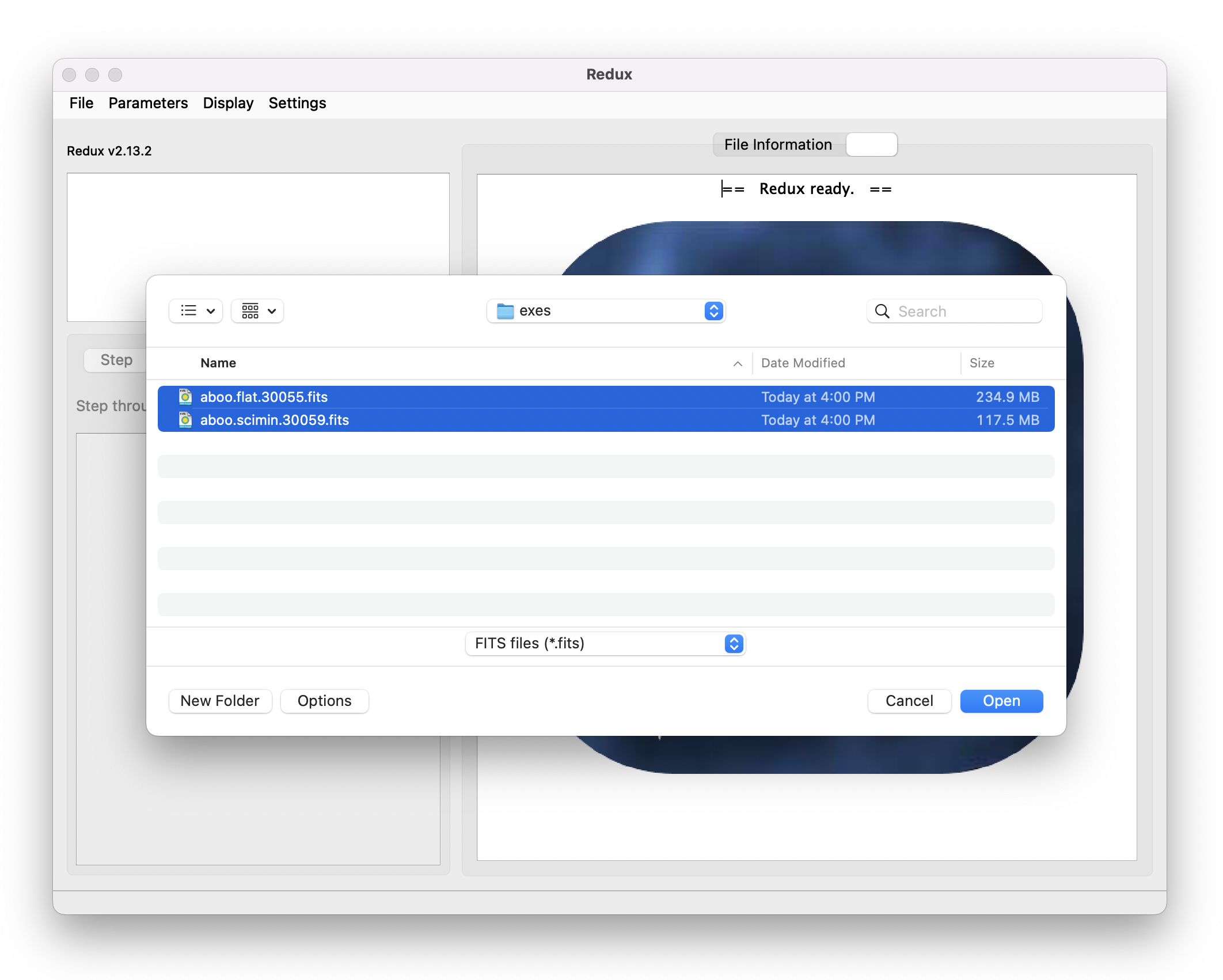
Fig. 10 Open new reduction.

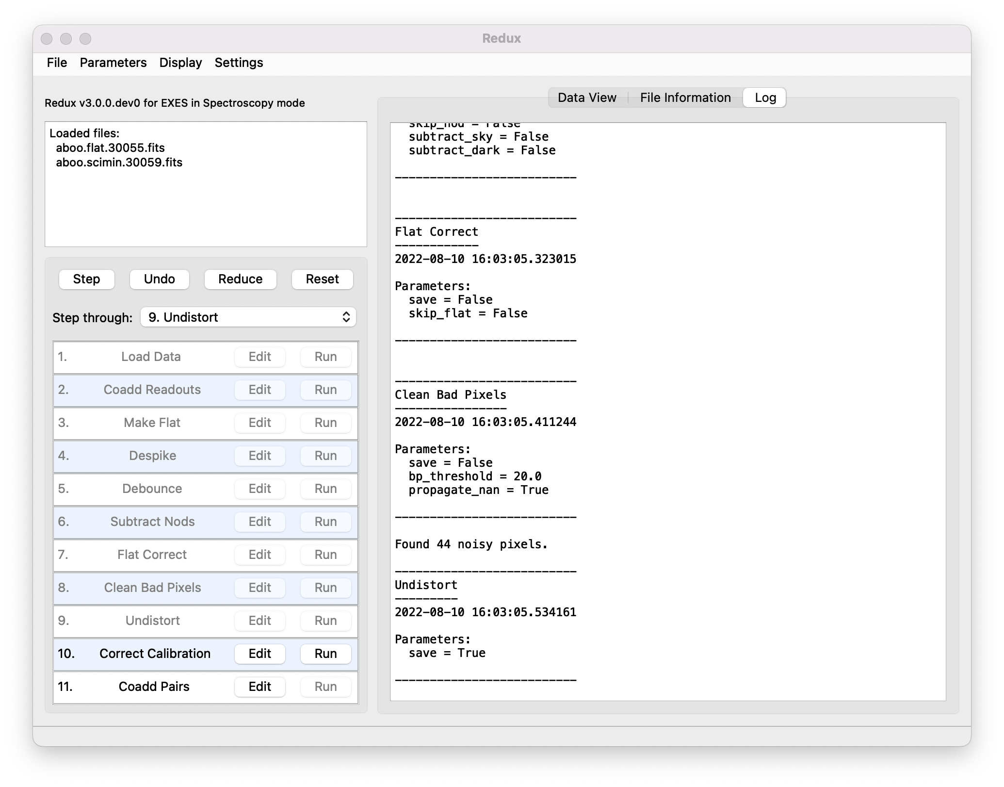
Fig. 11 Sample reduction steps. Log output from the pipeline is displayed in the Log tab.

Each reduction step has a number of parameters that can be edited before running the step. To examine or edit these parameters, click the Edit button next to the step name to bring up the parameter editor for that step (Fig. 12). Within the parameter editor, all values may be edited. Click OK to save the edited values and close the window. Click Reset to restore any edited values to their last saved values. Click Restore Defaults to reset all values to their stored defaults. Click Cancel to discard all changes to the parameters and close the editor window.

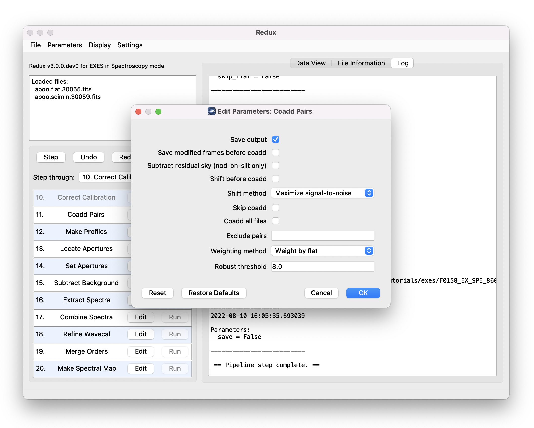
Fig. 12 Sample parameter editor for a pipeline step.

The current set of parameters can be displayed, saved to a file, or reset all at once using the Parameters menu. A previously saved set of parameters can also be restored for use with the current reduction (Parameters -> Load Parameters).

After all parameters for a step have been examined and set to the user’s satisfaction, a processing step can be run on all loaded files either by clicking Step, or the Run button next to the step name. Each processing step must be run in order, but if a processing step is selected in the Step through: widget, then clicking Step will treat all steps up through the selected step as a single step and run them all at once. When a step has been completed, its buttons will be grayed out and inaccessible. It is possible to undo one previous step by clicking Undo. All remaining steps can be run at once by clicking Reduce. After each step, the results of the processing may be displayed in a data viewer. After running a pipeline step or reduction, click Reset to restore the reduction to the initial state, without resetting parameter values.

Files can be added to the reduction set (File -> Add Files) or removed from the reduction set (File -> Remove Files), but either action will reset the reduction for all loaded files. Select the File Information tab to display a table of information about the currently loaded files (Fig. 13).

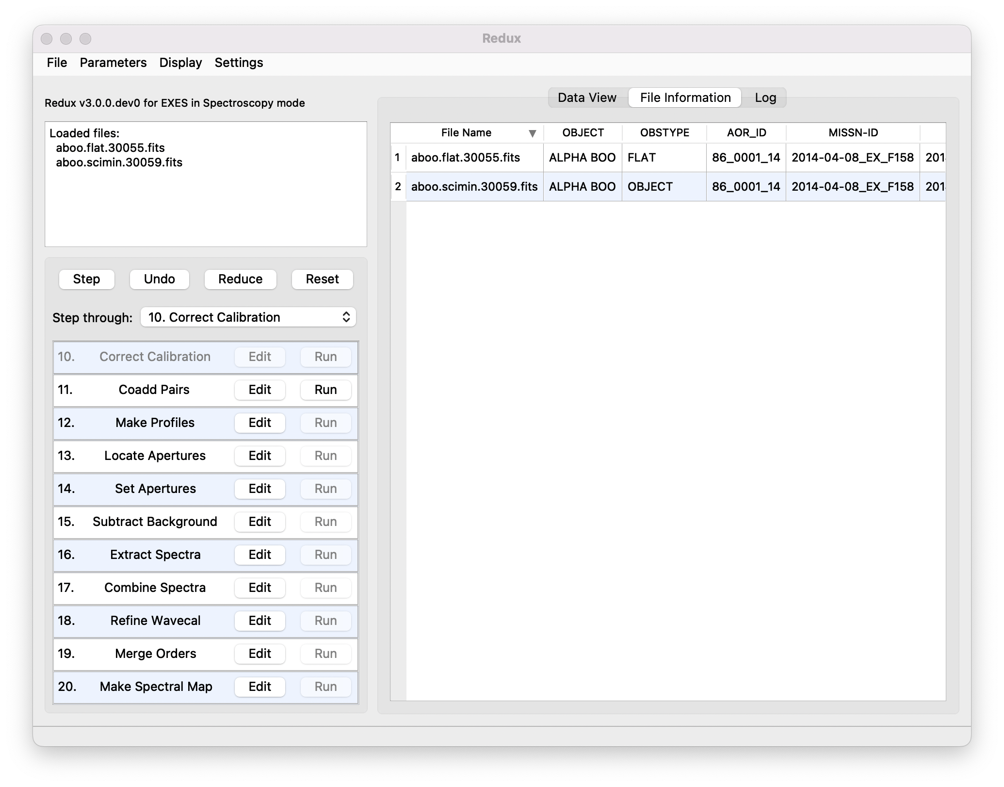
Fig. 13 File information table.

Display Features

The Redux GUI displays images for quality analysis and display (QAD) in the DS9 FITS viewer. DS9 is a standalone image display tool with an extensive feature set. See the SAO DS9 site (http://ds9.si.edu/) for more usage information.

After each pipeline step completes, Redux may load the produced images into DS9. Some display options may be customized directly in DS9; some commonly used options are accessible from the Redux interface, in the Data View tab (Fig. 14).

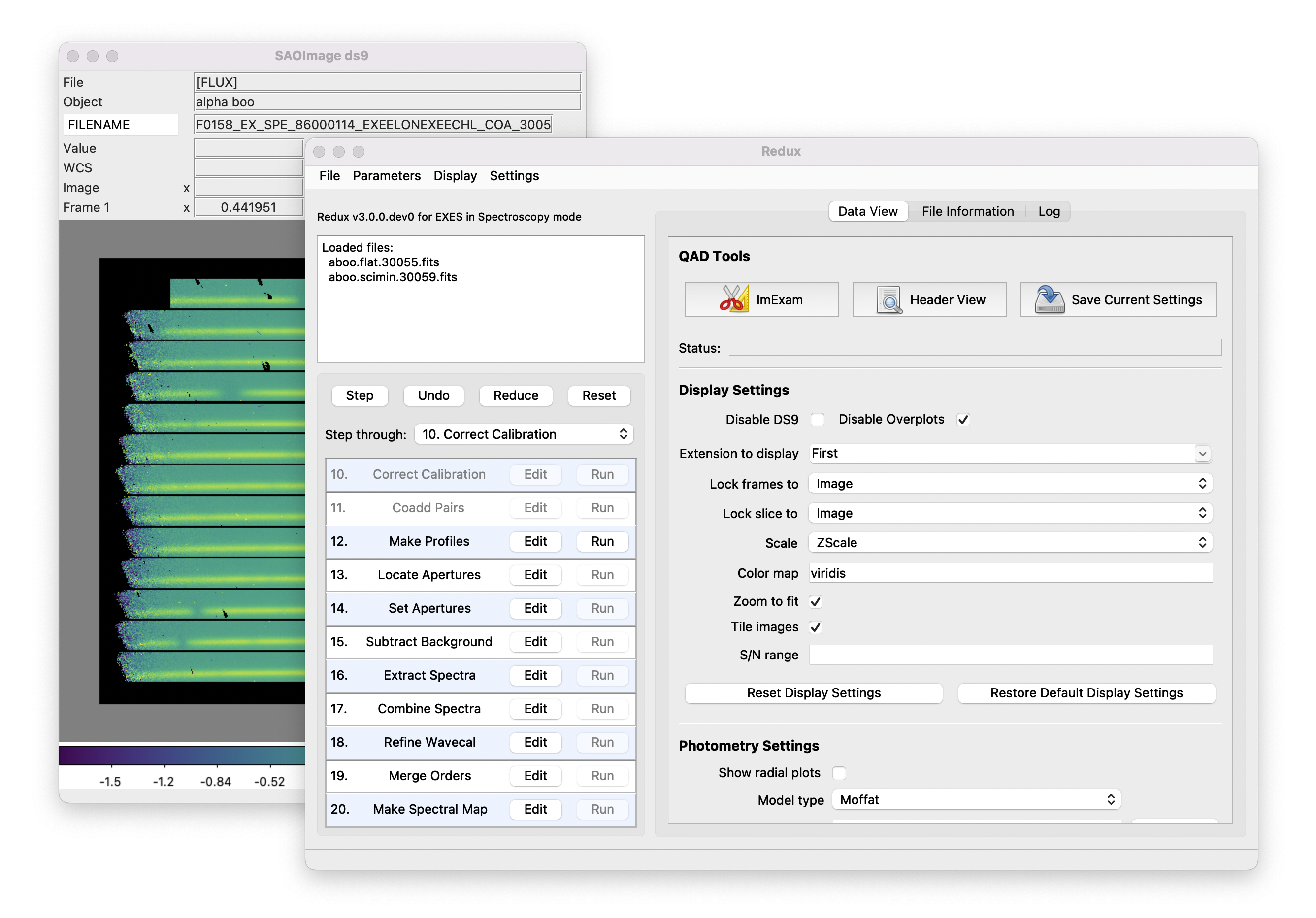
Fig. 14 Data viewer settings and tools.

From the Redux interface, the Display Settings can be used to:

• Set the FITS extension to display (First, or edit to enter a specific extension), or specify that all extensions should be displayed in a cube or in separate frames.

• Lock individual frames together, in image or WCS coordinates.

• Lock cube slices for separate frames together, in image or WCS coordinates.

• Set the image scaling scheme.

• Set a default color map.

• Zoom to fit image after loading.

• Tile image frames, rather than displaying a single frame at a time.

Changing any of these options in the Data View tab will cause the currently displayed data to be reloaded, with the new options. Clicking Reset Display Settings will revert any edited options to the last saved values. Clicking Restore Default Display Settings will revert all options to their default values.

In the QAD Tools section of the Data View tab, there are several additional tools available.

Clicking the ImExam button (scissors icon) launches an event loop in DS9. After launching it, bring the DS9 window forward, then use the keyboard to perform interactive analysis tasks:

• Type ‘a’ over a source in the image to perform photometry at the cursor location.

• Type ‘p’ to plot a pixel-to-pixel comparison of all frames at the cursor location.

• Type ‘s’ to compute statistics and plot a histogram of the data at the cursor location.

• Type ‘c’ to clear any previous photometry results or active plots.

• Type ‘h’ to print a help message.

• Type ‘q’ to quit the ImExam loop.

The photometry settings (the image window considered, the model fit, the aperture sizes, etc.) may be customized in the Photometry Settings. Plot settings (analysis window size, shared plot axes, etc.) may be customized in the Plot Settings. After modifying these settings, they will take effect only for new apertures or plots (use ‘c’ to clear old ones first). As for the display settings, the reset button will revert to the last saved values and the restore button will revert to default values. For the pixel-to-pixel and histogram plots, if the cursor is contained within a previously defined DS9 region (and the regions package is installed), the plot will consider only pixels within the region. Otherwise, a window around the cursor is used to generate the plot data. Setting the window to a blank value in the plot settings will use the entire image.

Clicking the Header button (magnifying glass icon) from the QAD Tools section opens a new window that displays headers from currently loaded FITS files in text form (Fig. 15). The extensions displayed depends on the extension setting selected (in Extension to Display). If a particular extension is selected, only that header will be displayed. If all extensions are selected (either for cube or multi-frame display), all extension headers will be displayed. The buttons at the bottom of the window may be used to find or filter the header text, or generate a table of header keywords. For filter or table display, a comma-separated list of keys may be entered in the text box.

Clicking the Save Current Settings button (disk icon) from the QAD Tools section saves all current display and photometry settings for the current user. This allows the user’s settings to persist across new Redux reductions, and to be loaded when Redux next starts up.

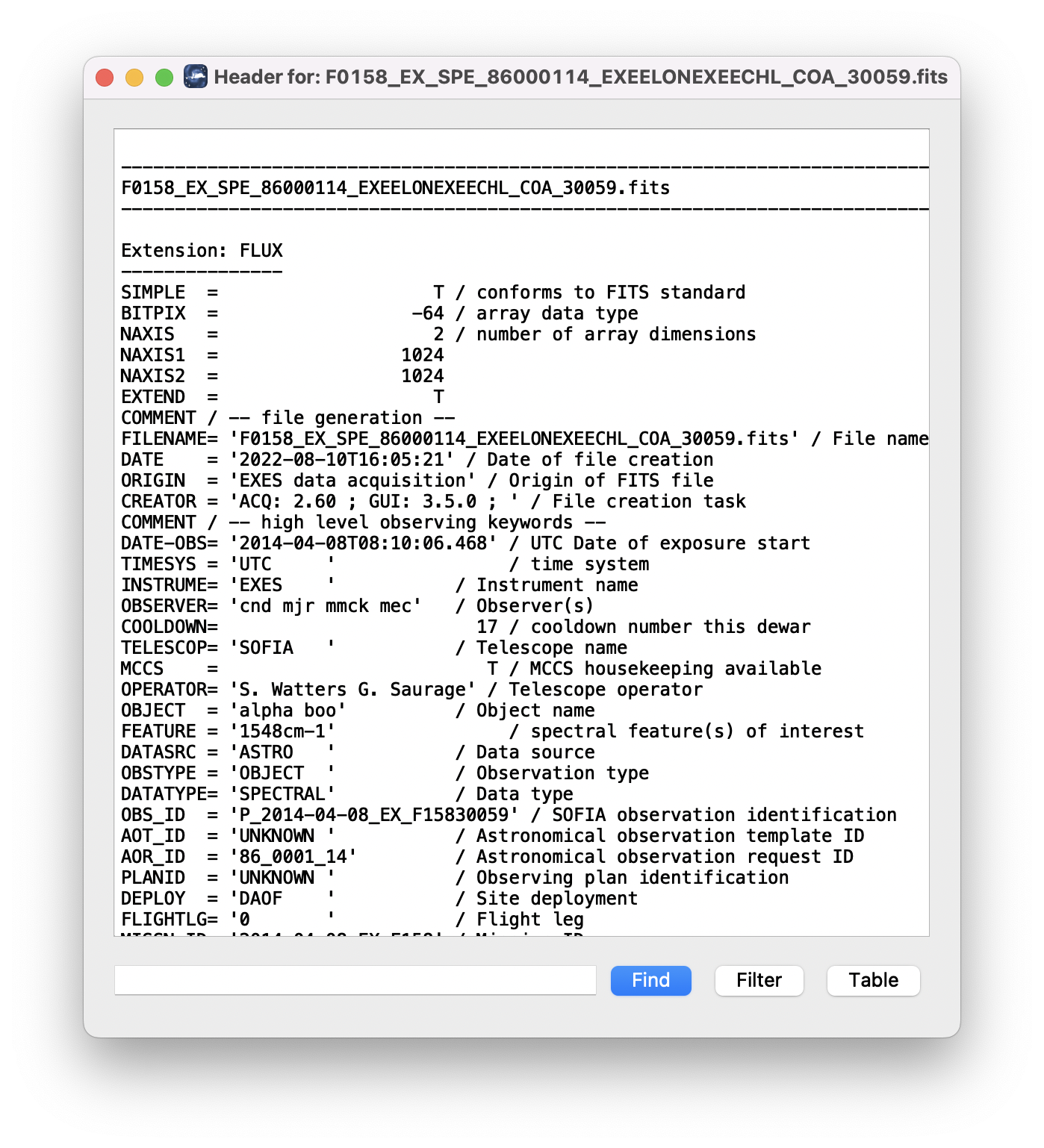
Fig. 15 QAD FITS header viewer.

EXES Reduction

EXES data reduction with Redux follows the data reduction flowchart in Fig. 1. At each step, Redux attempts to determine automatically the correct action, given the input data and default parameters, but each step can be customized as needed.

Image Processing

The early steps of the EXES pipeline are straightforward: the 2D images are processed to remove instrument and sky artifacts and calibrate to physical units. Their associated variances and reference data are propagated alongside the modified image in intermediate data products.

Spectroscopic Processing

Extraction Steps

Spectral extraction with Redux is slightly more complicated than image processing. The pipeline breaks down the spectral extraction algorithms into five separate reduction steps to give more control over the extraction process. These steps are:

• Make Profiles: Generate a smoothed model of the relative distribution of the flux across the slit (the spatial profile). After this step is run, a separate display window showing a plot of the spatial profile for each order appears.

• Locate Apertures: Use the spatial profile to identify spectra to extract. By default for most configurations, Redux attempts to automatically identify sources, but they can also be manually identified by entering a guess position to fit near, or a fixed position, in the parameters. Aperture locations are plotted in the profile window.

• Set Apertures: Identify the data to extract from the spatial profile. This is done automatically by default, but all aperture parameters can be overridden manually in the parameters for this step. Aperture radii and background regions are plotted in the profile window (see Fig. 16).

• Subtract Background: Residual background is fit and removed for each column in the 2D image, using background regions specified in the Set Apertures step.

• Extract Spectra: Extract one-dimensional spectra from the identified apertures. By default, Redux will attempt optimal extraction for most configurations. The method can be overridden in the parameters for this step.

EXES has a number of configurations for which either the source is too extended or the slit is too short to treat the target as a compact source. In particular, for high-low mode (unless nod-on-slit), for observations that are marked as extended sources (SRCTYPE=EXTENDED_SOURCE), or for sky spectra the default parameters are modified to:

• turn off median level subtraction in the spatial profile generation

• place a single aperture position at the center of the slit

• set the aperture radius to extract the full slit

• turn off background subtraction

• use standard extraction instead of optimal.

These defaults may still be overridden in the parameters for each step.

Spectral Displays

Extracted spectra are displayed in an interactive plot window, for data analysis and visualization (see Fig. 17).

The spectral display tool has a number of useful features and controls. See Fig. 18 and the table below for a quick summary.

Table 4 Spectral Viewer controls

Feature	Control	Keyboard shortcut
Load new FITS file	File Choice -> Add File	–
Remove loaded FITS file	File Choice -> Remove File	Press delete in the File Choice panel
Plot selected file	File Choice -> (double-click)	–
Add a new plot window (pane)	Panes -> Add Pane	–
Remove a pane	Panes -> Remove Pane	Press delete in the Panes panel, or in the plot window
Show or hide a plot	Panes -> Pane # -> File name -> Enabled, or click the Hide all/ Show all button	–
Display a different X or Y field (e.g. spectral error, transmission, or response)	Axis -> X Property or Y Property	–
Overplot a different Y axis field (e.g. spectral error, transmission, or response)	Axis -> Overplot -> Enabled	–
Change X or Y units	Axis -> X Unit or Y Unit	–
Change X or Y scale	Axis -> X Scale or Y Scale -> Linear or Log	–
Interactive zoom	Axis -> Zoom: X, Y, Box, then click in the plot to set the limits; or Reset to reset the limits to default.	In the plot window, press x, y, or z to start zoom mode in x-direction, y-direction, or box mode, respectively. Click twice on the plot to set the new limits. Press w to reset the plot limits to defaults.
Fit a spectral feature	–	In the plot window, press f to start the fitting mode. Click twice on the plot to set the data limits to fit.
Change the feature or baseline fit model	Analysis -> Feature, Background	–
Load a spectral line list for overplot display	Analysis -> Reference Data: Open, Load List Select a one- or two- column text file containing wavelengths in microns and (optionally) labels for the values. Columns may be comma, space, or ‘|’ separated.	–
Clear zoom or fit mode	–	In the plot window, press c to clear guides and return to default display mode.
Change the plot color cycle	Plot -> Color cycle -> Accessible, Spectral or Tableau	–
Change the plot type	Plot -> Plot type -> Step, Line, or Scatter	–
Change the plot display options	Plot -> Show markers, Show errors, Show grid, or Dark mode	–
Display the cursor position	Cursor panel -> Check Cursor Location for a quick display or press Popout for full information	–

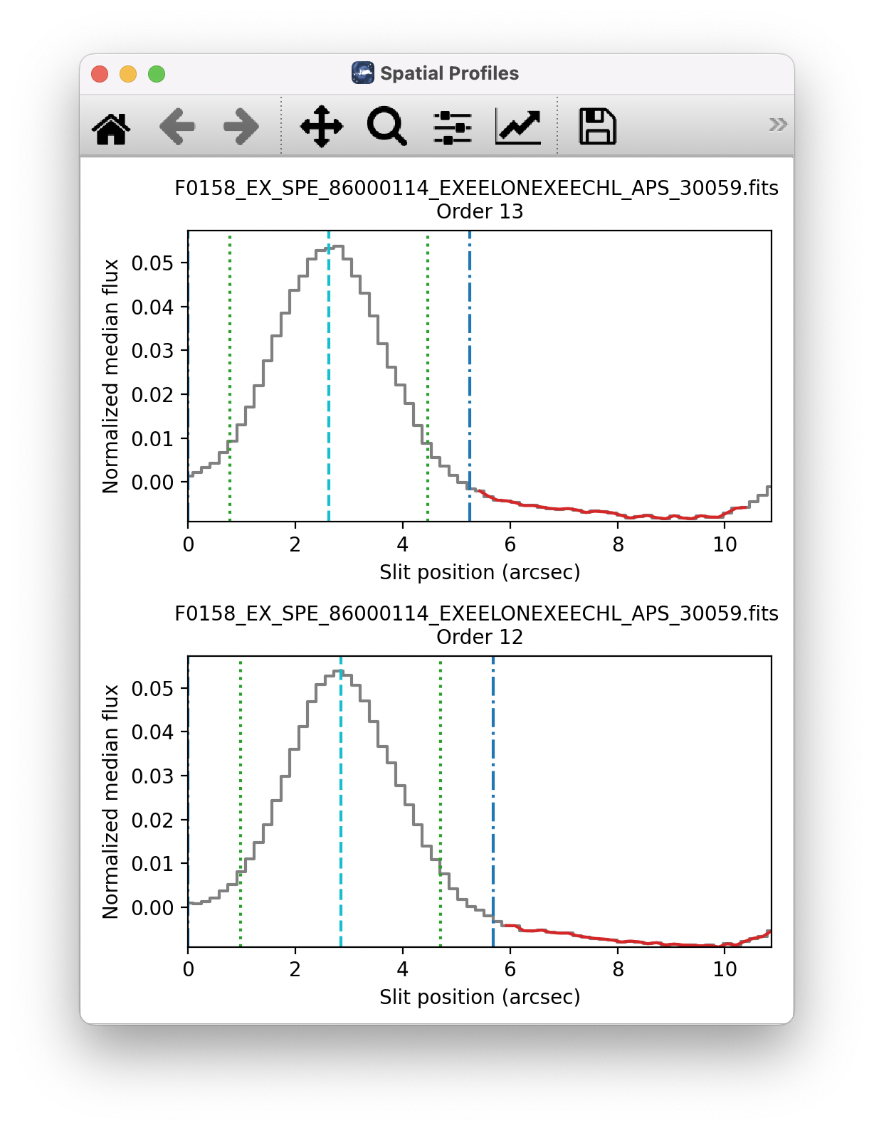
Fig. 16 Aperture location automatically identified and over-plotted on the spatial profile. The cyan line indicates the aperture center. Green lines indicate the integration aperture for optimal extraction, dark blue lines indicate the PSF radius (the point at which the flux goes to zero), and red lines indicate background regions.

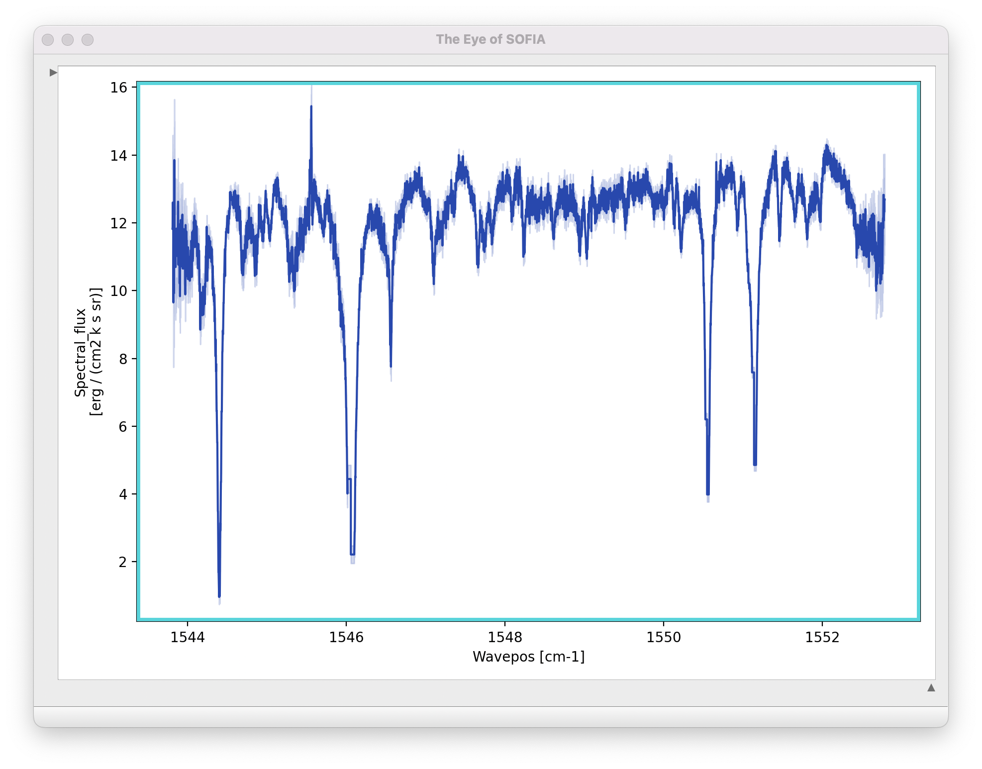
Fig. 17 Final extracted spectrum, displayed in an interactive plot window.

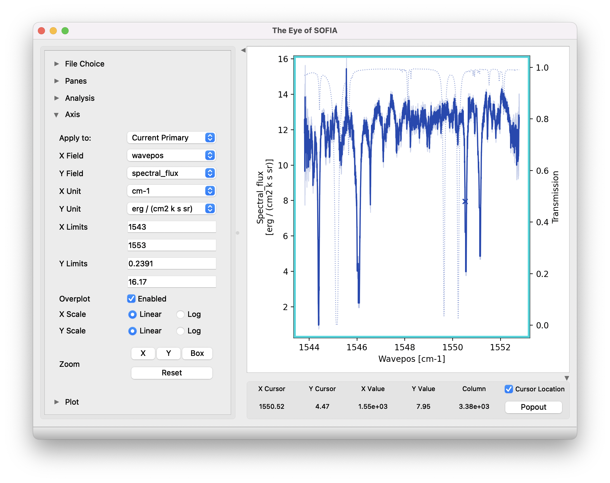
Fig. 18 Control panels for the spectral viewer are located to the left and below the plot window. Click the arrow icons to show or collapse them.

Useful Parameters

Some key parameters for all reduction steps are listed below.

In addition to the specified parameters, the output from each step may be optionally saved by selecting the ‘save’ parameter.

• Load Data:

  • Abort reduction for invalid headers: By default, Redux will abort the reduction if the input header keywords do not meet requirements. Unset this option to attempt the reduction anyway.

  • Extract sky spectrum: If set, the subsequent reduction will be treated as a sky extraction, for calibration purposes, rather than a science extraction. This will set the dark subtraction option in the Subtract Nods step, the ‘fix to center’ option in Locate Apertures, ‘extract the full slit’ option in Set Apertures, ‘skip background subtraction’ in Subtract Background, and extraction method: ‘standard’ in Extract Spectra. All output filenames and product types at and after the Subtract Nods step will be modified (see Table 2).

  • Central wavenumber: If the central wavenumber is known more precisely than the value in the WAVENO0 keyword, enter it here to use it in the distortion correction calculations and wavelength calibration. This value will be filled in automatically at the end of a reduction, if the Refine Wavecal step modifies the central wavenumber, so that the reduction may be reset and re-run with the new parameter.

  • HR focal length: This distortion parameter may be adjusted to tune the dispersion solution for cross-dispersed spectra. Reducing HRFL decreases the wavenumber of the left end of the order.

  • XD focal length: This distortion parameter may be adjusted to tune the dispersion solution for long-slit spectra. Reducing XDFL decreases the wavenumber of the left end of the order for a correctly identified central wavenumber. This parameter may also be adjusted to tune the predicted spacing between orders in cross-dispersed mode. In this case, increasing XDFL increases the predicted spacing.

  • Slit rotation: This distortion parameter may be adjusted to tune the slit skewing, to correct for spectral features that appear tilted across an order. For cross-dispersed modes, increasing the slit rotation angle rotates the lines clockwise in the undistorted image. For long-slit modes, decreasing the slit rotation angle rotates the lines clockwise in the undistorted image.

  • Detector rotation: This parameter may be adjusted to change the detector rotation from the default value.

  • HRR: This parameter may be adjusted to change the R number for the echelon grating.

  • Ambient temperature for the flat mirror: Set to override the default ambient temperature for the flat mirror. Typical default is 290K.

  • Emissivity for the flat mirror: Set to override the default emissivity fraction for the flat mirror. Typical default is 0.1.

• Coadd Readouts:

  • General Parameters

    • Readout algorithm: Set the readout mode. The default is ‘Last destructive only’, indicating that only the final destructive read should be used, regardless of readout pattern. ‘First/last’ will use the first non-destructive read and the last destructive; ‘Second/penultimate’ will use the second and second-to-last frames. ‘Default for read mode’ will attempt to choose the best read mode for the readout pattern used (typically Fowler mode).

    • Apply linear correction: If set, a standard linearity correction will be applied.

    • Correct odd/even row gains: If set, gain offsets between odd and even rows will be fit and removed.

  • Integration Handling Parameters

    • Science files: toss first integrations: If set to 0, all integration sets will be used. If set to 1 or 2, that many integrations will be discarded from the beginning of the raw input science files.

    • Flat files: toss first integrations: If set to 0, all integration sets will be used. If set to 1 or 2, that many integrations will be discarded from the beginning of the raw input flat files.

    • Dark files: toss first integrations: If set to 0, all integration sets will be used. If set to 1 or 2, that many integrations will be discarded from the beginning of the raw input dark files.

    • Copy integrations instead of tossing: If set, “tossed” integrations will be replaced with frames from the next B nod instead of discarded.

• Make Flat:

  • General Parameters

    • Save flat as separate file: The standard output from this step is the science files with flat planes attached. If this option is set, the flat information is additionally saved to a separate FITS file. This flat file may be used in place of raw flat files for future data reductions with the same instrument configuration.

  • Order Edge Determination Parameters

    • Threshold factor: This value defines the illumination threshold for a flat, which determines where the edges of cross-dispersed orders are placed. Enter a number between 0 and 1. If the pipeline reports that it can not determine order edges, increasing the threshold slightly, to widen the gaps between orders, may help.

    • Optimize rotation angle: Unset this option to prevent the pipeline from using the 2D FFT of the edge-enhanced flat to try to determine the best rotation angle (krot).

    • Edge enhancement method: Depending on the noise and illumination characteristics of the input flat, it may work better to take the 2D FFT of the squared derivative or the Sobel filtered image, rather than the derivative, of the flat. Use the drop-list to select an alternate algorithm.

    • Starting rotation angle: Enter a number here to use as the starting value for krot. If not set, the starting value will be taken from the default parameters in configuration tables.

    • Predicted spacing: Enter a value here, in pixels, to use as the predicted spacing for cross-dispersed orders. This number will be used as a first guess for the spacing parameter in the fit to the 2D FFT, overriding the value calculated from header parameters.

  • Order Edge Override Parameters

    • Bottom pixel for undistorted order: For medium and low configurations, specifying a value here sets the bottom edge of the order mask to this value.

    • Top pixel for undistorted order: Sets the top edge of the order mask to this value (medium and low only).

    • Starting pixel for undistorted order: Sets the left edge of all orders in the order mask to this value.

    • Ending pixel for undistorted order: Sets the right edges of all orders in the order mask to this value.

    • Custom cross-dispersed order mask: Select a file to directly define cross-dispersed order edges (bottom, top, start, and end). There should be one line for each order with edge values specified as white-space separated integers (B T S E), starting with the top-most order (largest B/T). Values are post-distortion correction and rotation, so that B/T are y values and S/E are x values, zero-indexed.

• Despike:

  • Combine all files before despike: If set, all planes from all files will be combined into a single file before computing outlier statistics. Input data will be treated as a single file for all subsequent steps.

  • Ignore beam designation: If set, all frames are used for computing outlier statistics, rather than comparing A nods and B nods separately.

  • Spike factor: Enter a value for the threshold for a pixel to be considered a spike. This value is multiplied by the standard deviation of the pixel across all frames: e.g. a value of 20 marks pixels with values over 20 sigma as bad pixels.

  • Mark trashed frames for exclusion: If set, frames that have significantly more noise compared to the rest will be identified and excluded from future processing. These frames will not be spike-corrected.

  • Propagate NaN values: If set, spiky pixels will be replaced with NaN values. If not, they will be replaced with the average value from the remaining frames.

• Debounce:

  • Bounce factor: Enter a number to use as the amplitude of the bounce correction. A value of 0 means no bounce correction will be applied. Values greater than 0 apply the first derivative bounce (shifting) only. Values less than 0 also apply the second derivative bounce (smoothing). Typical nonzero values are 0.1 or -0.1.

  • Spectral direction If set, the bounce correction will be applied in the spectral direction instead of the spatial direction.

• Subtract Nods:

  • Skip nod subtraction: If set, this option will cause the pipeline to continue without performing nod-subtraction. This option may be used to extract reference sky spectra.

  • Subtract residual sky: This option applies only to nod-off-slit mode. If set, it will attempt to remove any residual sky signal before subtracting pairs. This option will remove any average continuum value along the slit; if this is not desired, background regions should be set at the time of extraction instead.

  • Dark subtraction: If set, nod subtraction will be skipped and a dark frame will be subtracted from all planes instead. The dark file must have been loaded into the reduction with the raw data or attached to an input processed flat. If no dark is available, the step will fall back to skipping nod subtraction. This option may produce cleaner reference sky spectra than simply skipping nod subtraction.

• Flat Correct:

  • Skip flat correction: If set, the data will not be multiplied by the flat. This option is primarily used for testing.

• Clean Bad Pixels:

  • Bad pixel threshold: Enter a value for the threshold for a pixel to be considered a bad pixel. This value is multiplied by the standard deviation of all good pixels in the frame.

  • Propagate NaN values: If set, bad pixels are replaced with NaN and ignored in future processing steps. If not set, bad pixels are interpolated over.

• Undistort:

  • Interpolation method: Two interpolation methods are available for performing the distortion correction. ‘Cubic convolution’ replicates the behavior of the IDL interpolate function in the original pipeline, implementing a 2D separable parametric cubic convolution, with the edge-preserving parameter alpha set to -0.5 to mimic sinc interpolation. ‘Piecewise spline’ implements polynomial spline interpolation of specified order; cubic by default.

  • Spline order: Sets the polynomial order for piecewise spline interpolation. May be 0-5, where 0 is nearest value, 1 is linear, and 3 is cubic interpolation.

  • Set unilluminated pixels to NaN: If set, unilluminated areas of the flat field and order edges are set to NaN.

• Correct Calibration:

  • Skip calibration correction: If set, no calibration correction will be performed. This option is primarily used for testing.

• Coadd Pairs:

  • Save modified frames before coadd: If set, modified input data is saved to disk for inspection, prior to coadding. The output FITS file has file code COI and PRODTYPE = ‘coadd_input’.

  • Subtract residual sky: If set, the mean value at each wavelength bin will be subtracted to remove any residual sky noise. This option applies only to nod-on-slit mode.

  • Shift before coadd: Set to attempt to shift spectra in the spatial direction to align with each other before coadding.

  • Shift method: Select whether to maximize the signal or the signal-to-noise when determining the spatial shift.

  • Skip coadd: Check to skip coadding images and instead extract separate spectra from each frame. If selected, each frame will be treated as a separate file after this step. For map mode, coadding is skipped by default.

  • Coadd all files: If set, all input files will be coadded together, as if they were in a single file.

  • Exclude pairs: Enter comma-separated numbers to identify specific nod-subtracted frames to exclude from the coadd. For example, entering 1,4,7 will exclude the first, fourth, and seventh frame from the coadd. If multiple files are loaded, lists for each file may be entered, separated by a semi-colon. For example, 1,4;;3,10 will exclude the first and fourth frames for the first file and the third and tenth for the third file.

  • Robust threshold: Set to a number greater than zero to enable outlier rejection before coadding. The threshold value is the number of standard deviations away from the median for which a value is rejected.

  • Weighting method: Set to ‘uniform weights’ to use equal weights for all input frames. Otherwise, select ‘weight by flat’ to weight frames, using the flat illumination to determine good data, or ‘weight by variance’ to use the variance plane to identify good data.

  • Override weights: Enter comma-separated numbers to directly specify weight values for each input frame. Separate lists for multiple files with a semi-colon. If provided, the weighting method parameter is ignored.

• Convert units:

  • Skip unit conversion: If set, no flux unit conversion will be performed. This option is primarily used for testing.

  • Additional calibration scaling: If provided, this factor is multiplied into all flux extensions, for additional a priori calibration correction to the flux scale. This may be used to account for any known multiplicative systematic effects.

  • Additional calibration offset: If provided, this factor is added into all flux extensions after scaling, for additional a priori calibration correction to the flux zero level. This may be used to account for any known additive systematic effects.

• Make Profiles:

  • Row fit order: Typically a fourth-order polynomial fit is used to calculate the smooth spatial profile. Occasionally, a higher or lower order fit may give better results.

  • Subtract median background: If set, the median level of the smoothed spatial profile will be subtracted to remove residual background from the total extracted flux. This option is off by default for some modes (e.g. high-low data, sky spectra). For other data, this option is appropriate as long as the slit is dominated by background, rather than source flux. If the spatial profile dips below zero at any point (other than for a negative spectrum), this option should be deselected.

• Locate Apertures

  • Aperture location method: If ‘auto’, the strongest Gaussian peak(s) in the spatial profile will be selected, with an optional starting guess (Aperture position, below). If ‘fix to input’, the value in the Aperture position parameter will be used without refinement. If ‘fix to center’, the center of the slit will be used. ‘Fix to center’ is default for some modes (high-low data,sky spectra); otherwise ‘auto’ is default.

  • Number of auto apertures: Set this parameter to 1 to automatically find the single brightest source, or 2 to find the two brightest sources, etc. Sources may be positive or negative.

  • Aperture position: Enter a guess value for the aperture to use as a starting point for method = ‘auto’, or a fixed value to use as the aperture center for method = ‘fix to input’. Values are in arcseconds up the slit (refer to the spatial profile). Separate multiple apertures for a single file by commas; separate values for multiple files by semi-colons. For example, 3,8;2,7 will look for two apertures in each of two files, near 3” and 8” in the first image and 2” and 7” in the second image. If there are multiple files loaded, but only one aperture list is given, the aperture parameters will be used for all images.

  • Expected aperture FWHM (arcsec): Gaussian FWHM estimate for spatial profile fits, to determine peaks.

  • Exclude orders: Enter comma-separated numbers to identify specific orders to exclude from spectral extraction.

• Set Apertures:

  • Extract the full slit: If set, all other parameters are ignored, and the PSF radius will be set to include the full slit.

  • Refit apertures for FWHM: The spatial FWHM for the aperture is used to determine the aperture and PSF radii, unless they are directly specified. If this parameter is set, the profile will be re-fit with a Gaussian to determine the FWHM. If it is not set, the value determined or set in the Locate Apertures step is used (stored as APFWHM01 in the FITS header).

  • Aperture sign: Enter either 1 or -1 to skip the automatic determination of the aperture sign from the spatial profile. If the value is -1, the spectrum will be multiplied by -1. Separate multiple apertures by commas; separate values for multiple files by semi-colons. If a single value is specified, it will be applied to all apertures.

  • Aperture radius: Enter a radius in arcsec to skip the automatic determination of the aperture radius from the profile FWHM. Separate multiple apertures by commas; separate values for multiple files by semi-colons. If a single value is specified, it will be applied to all apertures.

  • PSF radius: Enter a radius in arcsec to skip the automatic determination of the PSF radius from the profile FWHM. Separate multiple apertures by commas; separate values for multiple files by semi-colons. If a single value is specified, it will be applied to all apertures.

  • Background regions: Enter a range in arcsec to use as the background region, skipping automatic background determination. For example, 0-1,8-10 will use the regions between 0” and 1” and between 8” and 10” to determine the background level to subtract in extraction. Values are for the full image, rather than for a particular aperture. Separate values for multiple files with semi-colons.

  • Override aperture start: Enter an aperture start location in arcsec. If set, and aperture end is also specified, this parameter overrides all other settings, including the starting aperture position.

  • Override aperture end: Enter an aperture end location in arcsec. If set, and aperture start is also specified, this parameter overrides all other settings, including the starting aperture position.

• Subtract Background

  • Skip background subtraction: Set to skip calculating and removing residual background. If no background regions were set, background subtraction will be automatically skipped.

  • Background fit order: Set to a number greater than or equal to zero for the polynomial order of the fit to the background regions.

  • Bad pixel threshold: Set to a value greater than or equal to zero to modify the robust threshold in the background fit.

• Extract Spectra

  • Save extracted 1D spectra: If set, the extracted spectra will be saved to disk in Spextool format (file code SPC, PRODTYPE = spectra_1d).

  • Extraction method: The default is to use standard extraction for EXTENDED_SOURCE, high-low data, and sky spectra; optimal extraction otherwise. Standard extraction may be necessary for some faint sources.

  • Use median profile instead of spatial map: By default, the pipeline uses a wavelength-dependent spatial map for extraction, but this method may give poor results if the signal-to-noise in the profile is low. Set this option to use the median spatial profile across all wavelengths instead.

  • Use spatial profile to fix bad pixels: The pipeline usually uses the spatial profile to attempt to interpolate over bad pixels during standard extraction, and in the output 2D image for either extraction method. Occasionally, this may result in a failed extraction. Unset this options to extract the spectra without bad pixel correction.

  • Bad pixel threshold: Enter a value for the threshold for a pixel to be considered a bad pixel. This value is multiplied by the standard deviation of all good pixels in the aperture at each wavelength bin.

  • ATRAN directory: This parameter specifies the location of a library of ATRAN FITS files to use. If blank or set to a directory that does not exist, the default files provided with the pipeline will be used.

  • ATRAN file: This parameter is used to directly override the ATRAN data to attach to the output spectrum, for reference. If blank, the default ATRAN file on disk will be used. Set to a valid FITS file path to override the default ATRAN file with a new one.

• Combine Spectra:

  • General Parameters

    • Combination method: Mean is the default for all data; median may also be useful for some input data.

    • Weight by errors: If set, the average of the data will be weighted by the errors. Ignored for method=median.

  • 1-2D Combination Parameters

    • Combine apertures: If unset, spectra from separate files will be combined, but separate apertures will remain separate in the output file.

    • Robust combination: If set, data will be sigma-clipped before combination for mean or median methods.

    • Outlier rejection threshold (sigma): The sigma-clipping threshold for robust combination methods, in units of sigma (standard deviation).

    • Maximum sigma-clipping iterations: The maximum number of rounds to use in outlier rejection.

• Refine Wavecal:

  • Order number for identified line: Enter an integer order number containing the identified spectral feature.

  • Identify line: Enter the pixel position of the spectral feature to use for refining the calibration.

  • Identify wavenumber: Enter the calibrated wavenumber of the identified spectral feature.

• Merge Orders:

  • General Parameters

    • ATRAN directory: This parameter specifies the location of a library of ATRAN FITS files to use. If blank or set to a directory that does not exist, the default files provided with the pipeline will be used.

    • ATRAN file: This parameter is used to directly override the ATRAN file to attach to the output spectrum, for reference. If blank, the default ATRAN file on disk will be used. Set to a valid FITS file path to override the default ATRAN file with a new one.

  • Trimming Parameters

    • Regions to trim before merge: Specified regions will be set to NaN before merging. Specify as semi-colon separated lists of order number : wavenumber regions. For example, “1:780-785,786-787;2:801.5-802.3” will trim 2 regions from order 1 and 1 region from order 2.

  • Merging Parameters

    • Selection threshold: By default, pixels in overlapping regions are used if their signal-to-noise ratio is greater than 0.1 times the maximum signal-to-noise in the order. Increasing or decreasing this value may reduce artifacts like discontinuous jumps or excessively noisy overlap regions. Set to 0 to turn off.

    • S/N statistic to compare: Sets the signal-to-noise statistic for use in rejecting pixels in overlapping regions. Default is ‘max’; ‘mean’ or ‘median’ may give more robust results in some cases.

    • Apply selection threshold to noise only: If set, the S/N statistic is computed from 1/noise only. This may be useful if there are large outliers in signal with low computed noise.

    • Use local standard deviation for noise thresholding: If set, the input error spectrum is ignored and a sliding standard deviation calculation is used in its place for S/N thresholding.

    • Radius for local standard deviation: Sets the window size for the sliding standard deviation calculation, in pixels.

• Make Spectral Map

  • Normalize spectrum before plotting: If set, the spectrum will be divided by its median value.

  • Flux scale for plot: Specify a low and high percentile value for the spectral flux scale, e.g. [0,99]. If set to [0, 100], Matplotlib defaults are used.

  • Fraction of outer wavelengths to ignore: Used to block edge effects for noisy spectral orders. Set to 0 to include all wavelengths in the plot.

  • Overplot transmission: If set, the atmospheric transmission spectrum will be displayed in the spectral plot.

  • Overplot error range: If set, the error spectrum is plotted as a range overlay.

  • Color map: Color map for the spectral plot colors. Any valid Matplotlib color map name may be specified.

  • Overplot color: Color for the transmission spectrum over plot. Any valid Matplotlib color value may be specified.

  • Watermark text: If set to a non-empty string, the text will be added to the lower-right of the image as a semi-transparent watermark.

Data quality assessment

After the pipeline has been run on a set of input data, the output products should be checked to ensure that the data has been properly reduced:

• Check the output to the terminal or the log for warnings or errors. Non-fatal warnings will be prepended with the string WARNING. Fatal errors will be prepended with the string ERROR.

• Check that the expected files were written to disk: there should, at a minimum, be a coadded 2D image (COA) and an extracted spectrum (MRD).

• Look at the reduced image. Check that the distortion correction appears to have been calculated and applied correctly: order edges and spectral lines should appear to be aligned with the image columns and rows. If they are not, there may be a problem with the flat or with the optical parameters used.

• Look at the intermediate extracted spectra in the spectral viewer. The spectra from positive and negative apertures should look similar. Spectra from separate observations of the same source in the same mode should look similar.

• Compare the signal-to-noise in the extracted spectrum to the reduced image. If the target seems bright in the reduced image, but the spectrum looks noisy, it may be that the aperture centers were not defined correctly.

• Check the aperture parameters recorded in the pipeline output and in the output file headers. The calculated aperture and PSF radii should have similar values for all apertures. The aperture centers for each order should also be similar in cross-dispersed spectra.

• Check the extracted spectra for excessive outliers. Most bad pixels should be removed in the extraction process. If they are not, it may be helpful to use the median spatial profile, set the bad pixel threshold lower, or manually trim noisy regions.

Appendix A: Sample configuration file

Below is a sample EXES Redux parameter override file in INI format. If present, the parameter value overrides the default defined by the EXES reduction object. If not present, the default value will be used.

# Redux parameters for EXES instrument in Spectroscopy mode
# Pipeline: EXES_REDUX v3_0_0
[1: load_data]
    abort = True
    sky_spec = False
    cent_wave = ""
    hrfl = ""
    xdfl = ""
    slit_rot = ""
    det_rot = ""
    hrr = ""
[2: coadd_readouts]
    save = True
    lin_corr = False
    toss_integrations = 0
    algorithm = Last destructive only
    refpix_bpm = default
[3: make_flat]
    save = False
    save_flat = True
    threshold = 0.15
    opt_rot = True
    edge_method = Derivative
    start_rot = ""
    predict_spacing = ""
    bottom_pix = ""
    top_pix = ""
    start_pix = ""
    end_pix = ""
    custom_wavemap = ""
[4: despike]
    save = False
    combine_all = False
    spike_fac = 20.0
    mark_trash = False
[5: debounce]
    save = False
    bounce_fac = 0.0
    spec_direction = False
[6: subtract_nods]
    save = False
    skip_nod = False
    subtract_sky = False
    subtract_dark = False
[7: flat_correct]
    save = False
    skip_flat = False
[8: clean_badpix]
    save = False
    bp_threshold = 20.0
    propagate_nan = True
[9: undistort]
    save = True
[10: correct_calibration]
    save = False
[11: coadd_pairs]
    save = True
    save_intermediate = False
    subtract_sky = False
    shift = False
    shift_method = Maximize signal-to-noise
    skip_coadd = False
    coadd_all_files = False
    exclude_pairs = ""
    weight_method = Weight by flat
    threshold = 8.0
[12: make_profiles]
    save = False
    fit_order = 4
    bg_sub = True
[13: locate_apertures]
    save = False
    method = auto
    num_aps = 1
    input_position = ""
    fwhm = 3.0
    exclude_orders = ""
[14: set_apertures]
    save = False
    full_slit = False
    refit = True
    apsign = ""
    aprad = ""
    psfrad = ""
    bgr = ""
    ap_start = ""
    ap_end = ""
[15: subtract_background]
    save = False
    skip_bg = False
    bg_fit_order = 0
    threshold = 4.0
[16: extract_spectra]
    save = True
    save_1d = True
    method = optimal
    use_profile = False
    fix_bad = True
    threshold = 5.0
    atrandir = $DPS_SHARE/calibrations/ATRAN/fits
    atranfile = ""
[17: combine_spectra]
    save = False
    method = mean
    weighted = True
    combine_aps = True
    robust = True
    threshold = 8.0
    maxiters = 5
[18: refine_wavecal]
    interactive = False
    identify_order = ""
    identify_line = ""
    identify_waveno = ""
[19: merge_orders]
    save = True
    threshold = 0.15
    trim = False
    trim_regions = ""
    atrandir = $DPS_SHARE/calibrations/ATRAN/fits
    atranfile = ""
[20: specmap]
    normalize = True
    scale = 0, 100
    ignore_outer = 0.0
    atran_plot = True
    error_plot = True
    colormap = plasma
    overplot_color = gray
    watermark = ""

Appendix B: Required Header Keywords

Sample EXES configuration file, typically located in sofia_redux/instruments/exes/data/header/headerdef.dat. Values marked with a Y in the reqd? column are keywords required to be present in input data. They must meet the type and range requirements listed for grouping and data reduction to be successful.

#
# This table lists keywords, allowed values, and defaults for
# all keywords to be written to output files.  Keywords
# required to be present in input files for correct data
# processing are marked with a 'Y'. A '.' in min, max, or enum
# means no requirement.  Some output keywords have defaults
# defined in other configuration files
#
# keyword  reqd?  default  type    min    max    enum
#-----------------------------------------------------------------
ADDTIME      N    -9999.   float   0.     .      .
AIRSPEED     N    -9999.   float   .      .      .
ALTI_STA     Y    -9999.   float   -60000 60000. .
ALTI_END     Y    -9999.   float   -60000 60000. .
AOR_ID       Y    UNKNOWN  string  .      .      .
AOT_ID       N    UNKNOWN  string  .      .      .
ASSC_AOR     N    UNKNOWN  string  .      .      .
ASSC_MSN     N    UNKNOWN  string  .      .      .
ASSC_OBS     N    UNKNOWN  string  .      .      .
BB_TEMP      Y    273.16   float   1      9999.  .
BEAMTIME     N    0.0      float   .      .      .
BNU_T        N    -9999.   float   .      .      .
BOUNCE       N    0.0      float   .      .      .
BPM          N    UNKNOWN  string  .      .      .
BRL          N    -9999.   float   .      .      .
CARDMODE     N    BLKSKY   string  .      .      NONE|BLK|SKY|SHINY|BLKSKY|BLKSHINY|BLKOBJ|OBJ
CHOPPING     N    F        bool    .      .      .
CREATOR      N    UNKNOWN  string  .      .      .
CUMTIME      N    -9999.   float   0.     .      .
DARKVAL      N    0.       float   0.     .      .
DATAPATH     N    UNKNOWN  string  .      .      .
DATASRC      Y    UNKNOWN  string  .      .      ASTRO|CALIBRATION|LAB|TEST|OTHER|FIRSTPOINT
DATATYPE     N    UNKNOWN  string  .      .      IMAGE|SPECTRAL|OTHER
DATE         N    UNKNOWN  string  .      .      .
DATE-OBS     Y    UNKNOWN  string  .      .      .
DEPLOY       N    UNKNOWN  string  .      .      .
DETECTOR     N    UNKNOWN  string  .      .      .
DETROT       N    -9999.   float   .      .      .
DETSEC       N    UNKNOWN  string  .      .      .
DETSIZE      N    UNKNOWN  string  .      .      .
DITHER       N    F        bool    .      .      .
DRKFILE      N    UNKNOWN  string  .      .      .
DTHINDEX     N    -9999    int     .      .      .
DTHNPOS      N    -9999    int     .      .      .
DTHOFFS      N    -9999.   float   .      .      .
DTHPATT      N    UNKNOWN  string  .      .      3-POINT|5-POINT|9-POINT|CUSTOM
ECHELLE      Y    60.0     float   -35.   70.    .
ECTPAT       Y    UNKNOWN  string  .      .      .
EFL          N    -9999.   float   .      .      .
EFL0         N    -9999.   float   .      .      .
EPERADU      Y    75.0     float   1.     9999.  .
EQUINOX      N    -9999.   float   .      .      .
EXCLUDE      N    None     string  .      .      .
EXPTIME      N    -9999.   float   0.     .      .
FBC-STAT     N    UNKNOWN  string  .      .      FBC_OFF|FBC_QS|FBC_DY|FBC_ON
FDATE        N    0.0      float   0.     9999.  .
FILENAME     Y    UNKNOWN  string  .      .      .
FILENUM      N    .        string  .      .      .
FILEREV      N    UNKNOWN  string  .      .      .
FLIGHTLG     N    UNKNOWN  string  .      .      .
FOCUS_EN     N    -9999.   float   -5000  5000   .
FOCUS_ST     N    -9999.   float   -5000  5000   .
FRAMETIM     Y    1.0      float   0.     9999.  .
GRATANGL     N    0.0      float   -360.  360.   .
GRDSPEED     N    -9999.   float   .      .      .
HEADING      N    -9999.   float   .      .      .
HEADSTAT     N    UNKNOWN  string  .      .      ORIGINAL|UNKNOWN|CORRECTED|ERROR|MODIFIED
HRDGR        N    0.7588   float   .      .      .
HRFL         N    -9999.   float   .      .      .
HRFL0        N    -9999.   float   .      .      .
HRG          N    -0.015   float   .      .      .
HRR          N    -9999.   float   .      .      .
IMAGEID      N    -9999    int     0      .      .
INSTCFG      Y    UNKNOWN  string  .      .      HI-MED|MED|HI-LO|LO|CAM|PUP|HIMED|HILOW|LOW|CAMERA|HIGH_MED|HIGH_LOW|MEDIUM|HIGH-MED|HIGH-LOW
INSTMODE     Y    UNKNOWN  string  .      .      STARE|NOD_ON_SLIT|NOD_OFF_SLIT|MAP
INSTRUME     Y    EXES     string  .      .      EXES|TEXES
KROT         N    -9999.   float   .      .      .
KWDICT       N    UNKNOWN  string  .      .      .
LASTREW      N    UNKNOWN  string  .      .      .
LAT_STA      N    -9999.   float   .      .      .
LAT_END      N    -9999.   float   .      .      .
LINFILE      N    UNKNOWN  string  .      .      .
LO_LIM       N    0.0      float   .      .      .
LON_STA      N    -9999.   float   .      .      .
LON_END      N    -9999.   float   .      .      .
MAPCRSYS     N    UNKNOWN  string  .      .      EQUATORIAL|GALACTIC|ECLIPTIC|USER
MAPINTX      N    -9999.   float   .      .      .
MAPINTY      N    -9999.   float   .      .      .
MAPNXPOS     N    -9999    int     .      .      .
MAPNYPOS     N    -9999    int     .      .      .
MAPPING      N    F        bool    .      .      .
MCCSMODE     N    UNKNOWN  string  .      .      .
MISSN-ID     Y    UNKNOWN  string  .      .      .
NBELOW       N    -9999    int     0      .      .
NAIF_ID      N    .        int     .      .      .
NEXP         N    -9999    int     1      .      .
NFRAME       N    -9999    int     1      .      .
NINT         Y    1        int     1      .      .
NODAMP       N    -9999.   float   .      .      .
NODANGLE     N    -9999.   float   -180   180    .
NODBEAM      N    UNKNOWN  string  .      .      .
NODCRSYS     N    UNKNOWN  string  .      .      ERF|ECRF|GALRF|TARF|FPIRF|FFIRF|WFIRF|SIRF|USER
NODDING      N    F        bool    .      .      .
NODN         N    -9999    int     .      .      .
NODPATT      N    UNKNOWN  string  .      .      ABBA|AB|CUSTOM
NODSETL      N    -9999.   float   .      .      .
NODSTYLE     N    UNKNOWN  string  .      .      NMC|NPC|C2NC2|CUSTOM
NODTIME      N    -9999.   float   .      .      .
NORDERS      N    -9999    int     0      9999   .
NSPAT        N    1024     int     0      1025   .
NSPEC        N    1024     int     0      1025   .
NSUM         N    1        int     0      9999   .
NT           N    1024     int     0      1024   .
OBJECT       Y    UNKNOWN  string  .      .      .
OBS_ID       Y    UNKNOWN  string  .      .      .
OBSDEC       N    -9999.   float   -90.   90.    .
OBSERVER     N    UNKNOWN  string  .      .      .
OBSRA        N    -9999.   float   0.     24.    .
OBSTYPE      Y    UNKNOWN  string  .      .      OBJECT|STANDARD_FLUX|STANDARD_TELLURIC|LAMP|FLAT|DARK|BIAS|SKY
OMEGAP       N    -9999.   float   .      .      .
OPERATOR     N    UNKNOWN  string  .      .      .
ORDR_B       N    UNKNOWN  string  .      .      .
ORDR_T       N    UNKNOWN  string  .      .      .
ORDR_S       N    UNKNOWN  string  .      .      .
ORDR_E       N    UNKNOWN  string  .      .      .
ORIGIN       N    UNKNOWN  string  .      .      .
OTPAT        Y    UNKNOWN  string  .      .      .
PAGAIN       Y    1.0      float   0.     9999.  .
PINHOLE      N    0        int     -1     2      .
PIPELINE     N    UNKNOWN  string  .      .      .
PIPEVERS     N    UNKNOWN  string  .      .      .
PIXELWD      N    0.0025   float   0.     9999.  .
PIXSCAL      N    -9999.   float   .      .      .
PKGPATH      N    UNKNOWN  string  .      .      .
PLANID       Y    UNKNOWN  string  .      .      .
PLTSCALE     N    -9999.   float   .      .      .
PROCSTAT     Y    UNKNOWN  string  .      .      .
PRODTYPE     N    UNKNOWN  string  .      .      .
RAWFNAME     N    .        string  .      .      .
READNOIS     N    30.      float   0.     9999.  .
RESOLUN      N    -9999.   float   .      .      .
SATVAL       N    16000.   float   0.     65536  .
SCANNING     N    F        bool    .      .      .
SDEG         Y    180.     float   -45.   405.   .
SIBS_X       N    -9999    int     .      .      .
SIBS_Y       N    -9999    int     .      .      .
SLIT         Y    UNKNOWN  string  .      .      .
SLITOFF      N    -0.3     float   .      .      .
SLITROT      N    -9999.   float   .      .      .
SLITVAL      N    -9999.   float   .      .      .
SLITWID      N    -9999.   float   .      .      .
SPACING      N    -9999.   float   .      .      .
SPECTEL1     Y    UNKNOWN  string  .      .      .
SPECTEL2     Y    UNKNOWN  string  .      .      .
SPIKEFAC     N    20.0     float   0.     9999.  .
SRCTYPE      Y    UNKNOWN  string  .      .      POINT_SOURCE|EXTENDED_SOURCE|OTHER|UNKNOWN
STDFAC       N    20.0     float   0.     9999.  .
SUBARRNO     N    -9999    int     .      .      .
TELCONF      N    UNKNOWN  string  .      .      .
TELDEC       N    -9999.   float   -90.   90.    .
TELEL        N    -9999.   float   0.     90.    .
TELEQUI      N    UNKNOWN  string  .      .      .
TELESCOP     N    UNKNOWN  string  .      .      .
TELLOS       N    -9999.   float   -180   180    .
TELRA        N    -9999.   float   0.     24.    .
TELVPA       N    -9999.   float   0.     360.   .
TELXEL       N    -9999.   float   -90.   90.    .
TEMP_OUT     N    -9999.   float   .      .      .
TEMPPRI1     N    -9999.   float   -273.  .      .
TEMPPRI2     N    -9999.   float   -273.  .      .
TEMPPRI3     N    -9999.   float   -273.  .      .
TEMPSEC1     N    -9999.   float   .      .      .
THRFAC       N    0.5      float   0.     1.001  .
TRACERR      N    F        bool    .      .      .
TRACKANG     N    -9999.   float   .      .      .
TRACMODE     N    UNKNOWN  string  .      .      OFF|CENTROID|ROF|LIMB| OFFSET|ROF+OFFSET|CENTROID+INERTIAL|ROF+INERTIAL|OFFSET+INERTIAL|ROF+OFFSET+INERTIAL
TRASH        N    100.0    float   .      .      .
TSC-STAT     N    UNKNOWN  string  .      .      .
UP_LIM       N    11000.0  float   .      .      .
UTCSTART     N    UNKNOWN  string  .      .      .
UTCEND       N    UNKNOWN  string  .      .      .
WAVECENT     Y    0.0      float   0.     .      .
WAVENO0      Y    0.0      float   0.     .      .
WNO0         N    -9999.   float   0.     .      .
WVZ_STA      N    -9999.   float   0.     .      .
WVZ_END      N    -9999.   float   0.     .      .
X0BRL        N    -9999.   float   .      .      .
XD0          N    0.0      float   .      .      .
XDDELTA      N    0.0235   float   .      .      .
XDDGR        N    -9999.   float   .      .      .
XDFL         N    -9999.   float   .      .      .
XDFL0        N    -9999.   float   .      .      .
XDG          N     0.033   float   .      .      .
XDLRDGR      N    0.001328 float   .      .      .
XDMRDGR      N    0.003151 float   .      .      .
XDR          N    -9999.   float   .      .      .
XORDER1      N    0.0      float   0.     1024   .
Y0BRL        N    -9999.   float   .      .      .
ZA_START     Y    -9999.   float   -99999 90.    .
ZA_END       Y    -9999.   float   -99999 90.    .

Appendix B: Change notes for the EXES pipeline

Significant changes

Below are listed the most significant changes for the EXES pipeline over its history, highlighting impacts to science data products. See the data handbooks or user manuals associated with each release for more information.

All pipeline versions prior to v3.0.0 were implemented in IDL; v3.0.0 and later were implemented in Python. For previously processed data, check the PIPEVERS keyword in the FITS header to determine the pipeline version used.

EXES Redux v3.0.0 (2022-12-13)

User manual: Rev. E

• Full reimplementation of the IDL pipeline into Python 3.

• All intermediate and final data products were revised to separate flux, error, and calibration information into separate extensions in the output FITS files.

• Added a calibration correction step to account for wavenumber dependence in the blackbody calibration. Additionally, modified blackbody calibration to account for an extra contribution from flat mirror reflection.

• Added conversion to flux units (Jy/pixel for 2D images; Jy for 1D spectra) as a separate step, following nod-pair coaddition.

• Allowed despike comparison to be performed across all input files for better statistics in truncated observations.

• Allowed NaN propagation for bad pixel identification, rather than requiring immediate interpolation.

• Cross-dispersed data are rotated to align spectra with image rows immediately after distortion correction, prior to coaddition and extraction.

• Added a reference response spectrum, extracted from flat data at the same location as the science and attached to 1D spectral products as a 5th row.

• Added handling for resolution value configuration tables for cross-dispersed modes.

• Replaced ATRAN reference atmospheric spectra with Planetary Spectrum Generator (PSG) model files.

• Time keywords EXPTIME, INTTIME, and TOTTIME were revised to reflect nominal on-source time, integration time, and total elapsed time, respectively.

EXES Redux v2.2.0 (2022-04-06)

User manual: Rev. D

• Added HRR and DETROT to distortion correction parameters in configuration files, so that the defaults can be overridden by date.

• Fixed a bug in integration tossing in the initial read and coadd, in the case where a single valid integration remains after tossing bad ones.

EXES Redux v2.1.0 (2021-11-22)

User manual: Rev. C

• Designated separate product names and types for sky spectra to avoid overwriting science products.

• Added additional support for intermediate reductions, including sky spectrum products and undistorted files.

• Added capability to compose flat fields from separate subarrays (rasters).

• Modified assumed plate scale by mode to more accurately reflect anamorphic magnification effects for cross-dispersed modes.

EXES Redux v2.0.0 (2021-10-21)

User manual: Rev. B

• Adopted EXES PI team version for SOFIA DPS support as a facility class instrument.

• Modified NAIF ID handling to not write default -9999 value for sidereal targets.

• Added option to coadd frames across all files with outlier rejection.

• Added ASSC_MSN keyword to track all input mission IDs and ASSC_OBS to track all input OBS-IDs.

• Removed a scaling factor in the coadd step, originally intended for unit conversion and flux conservation, that was historically inconsistently applied to flux and variance planes.

EXES Redux v1.6.0 (2019-04-02)

User manual: Rev. A

• Added handling for darks to allow for black-dark flat generation method

• Added option to reject 1 or 2 initial readout patterns before readout coadd

• Added option to use only destructive frames for readout coadds

• Modified options to allow manual selection of bad pixel masks

• Allowed manual overrides for the edges of order masks

• Added option to debounce in the spectral direction, as well as the spatial

• Added manual options to set asymmetric apertures with start and end values

• Added options to subtract a dark frame instead of nods, for sky emission spectra

EXES Redux v1.0.2 (2015-07-17)

User manual: Rev. A

• Modified nonlinearity correction to allow for a lower-limit plane in the coefficient reference file.

EXES Redux v1.0.1 (2015-05-14)

User manual: Rev. -

• Added ASSC_AOR keyword to track all input AOR-IDs.

• Attached reference atmospheric transmission data to spectra.

• Improved wavelength calibration.

EXES Redux v1.0.0 (2015-03-17)

User manual: Rev. -

• Initial release.