HAWC+ DRP User’s Manual

Introduction

The SI Pipeline User’s Manual (OP10) is intended for use by both SOFIA Science Center staff during routine data processing and analysis, and also as a reference for Guest Observers (GOs) and archive users to understand how the data in which they are interested was processed. This manual is intended to provide all the needed information to execute the SI data reduction pipeline, and assess the data quality of the resulting products. It will also provide a description of the algorithms used by the pipeline and both the final and intermediate data products.

A description of the current pipeline capabilities, testing results, known issues, and installation procedures are documented in the SI Pipeline Software Version Description Document (SVDD, SW06, DOCREF). The overall Verification and Validation (V&V) approach can be found in the Data Processing System V&V Plan (SV01-2232). Both documents can be obtained from the SOFIA document library in Windchill.

This manual applies to HAWC DRP version 3.2.0.

SI Observing Modes Supported

HAWC+ Instrument Information

HAWC+ is the upgraded and redesigned incarnation of the High-Resolution Airborne Wide-band Camera instrument (HAWC), built for SOFIA. Since the original design never collected data for SOFIA, the instrument may be alternately referred to as HAWC or HAWC+. HAWC+ is designed for far-infrared imaging observations in either total intensity (imaging) or polarimetry mode.

HAWC currently consists of dual TES BUG Detector arrays in a 64x40 rectangular format. A six-position filter wheel is populated with five broadband filters ranging from 40 to 250 \(\mu\)m and a dedicated position for diagnostics. Another wheel holds pupil masks and rotating half-wave plates (HWPs) for polarization observations. A polarizing beam splitter directs the two orthogonal linear polarizations to the two detectors (the reflected (R) array and the transmitted (T) array). Each array was designed to have two 32x40 subarrays, for four total detectors (R0, R1, T0, and T1), but T1 is not currently available for HAWC. Since polarimetry requires paired R and T pixels, it is currently only available for the R0 and T0 arrays. Total intensity observations may use the full set of 3 subarrays.

HAWC+ Observing Modes

The HAWC instrument has two instrument configurations, for imaging and polarization observations. In both types of observations, removing background flux due to the telescope and sky is a challenge that requires one of several observational strategies. The HAWC instrument may use the secondary mirror to chop rapidly between two positions (source and sky), may use discrete telescope motions to nod between different sky positions, or may use slow continuous scans of the telescope across the desired field. In chopping and nodding strategies, sky positions are subtracted from source positions to remove background levels. In scanning strategies, the continuous stream of data is used to solve for the underlying source and background structure.

The instrument has two standard observing modes for imaging: the Chop-Nod instrument mode combines traditional chopping with nodding; the Scan mode uses slow telescope scans without chopping. The Scan mode is the most commonly used for total intensity observations. Likewise, polarization observations may be taken in either Nod-Pol or Scan-Pol mode. Nod-Pol mode includes chopping and nodding cycles in multiple HWP positions; Scan-Pol mode includes repeated scans at multiple HWP positions.

All modes that include chopping or nodding may be chopped and nodded on-chip or off-chip. Currently, only two-point chop patterns with matching nod amplitudes (nod-match-chop) are used in either Chop-Nod or Nod-Pol observations, and nodding is performed in an A-B-B-A pattern only. All HAWC modes can optionally have a small dither pattern or a larger mapping pattern, to cover regions of the sky larger than HAWC’s fields of view. Scanning patterns may be either box rasters or Lissajous patterns.

Algorithm Description

Chop-Nod and Nod-Pol Reduction Algorithms

The following sections describe the major algorithms used to reduce Chop-Nod and Nod-Pol observations. In nearly every case, Chop-Nod (total intensity) reductions use the same methods as Nod-Pol observations, but either apply the algorithm to the data for the single HWP angle available, or else, if the step is specifically for polarimetry, have no effect when called on total intensity data. Since nearly all total intensity HAWC observations are taken with scanning mode, the following sections will focus primarily on Nod-Pol data.

See the figures below for flow charts that illustrate the data reduction process for Nod-Pol data (Fig. 100 and Fig. 101) and Chop-Nod data (Fig. 102 and Fig. 103).

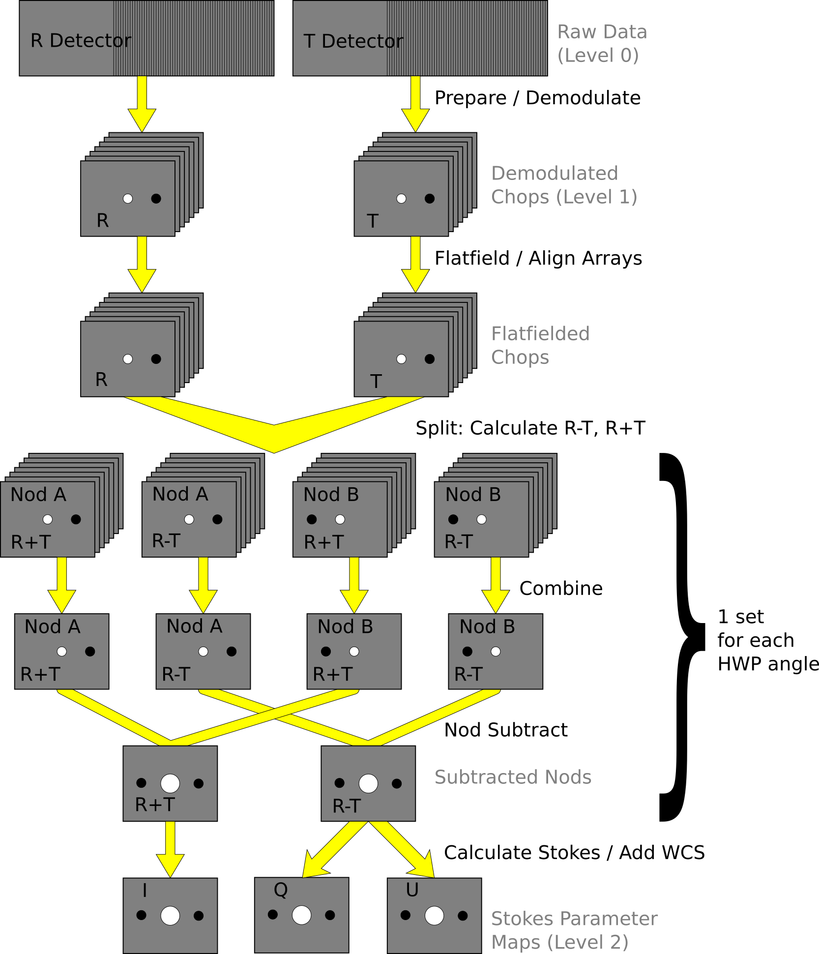
Fig. 100 Nod-Pol data reduction flowchart, up through Stokes parameter calculation for a single input file.

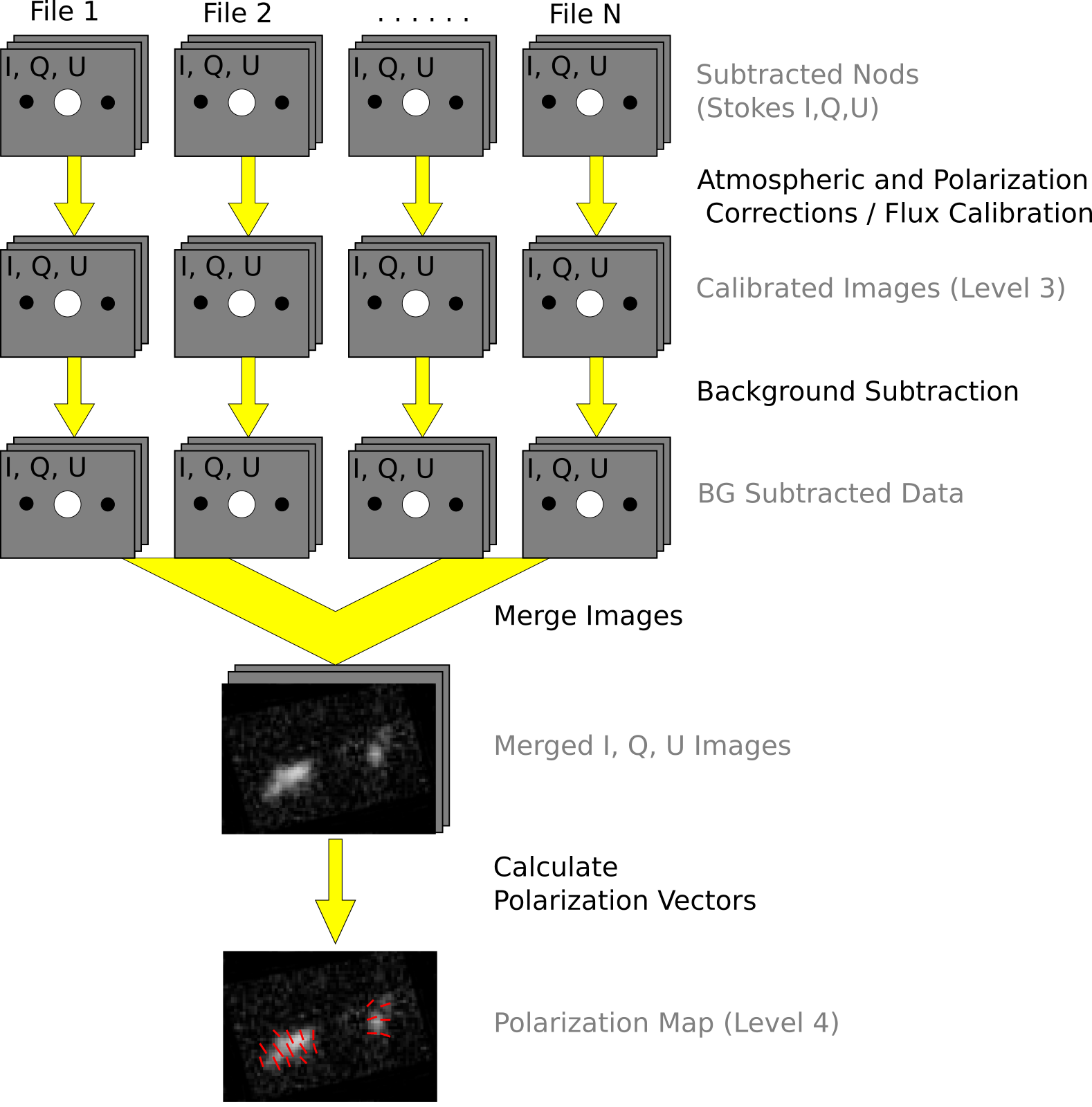
Fig. 101 Nod-Pol data reduction flowchart, picking up from Stokes parameter calculation, through combining multiple input files and calculating polarization vectors.

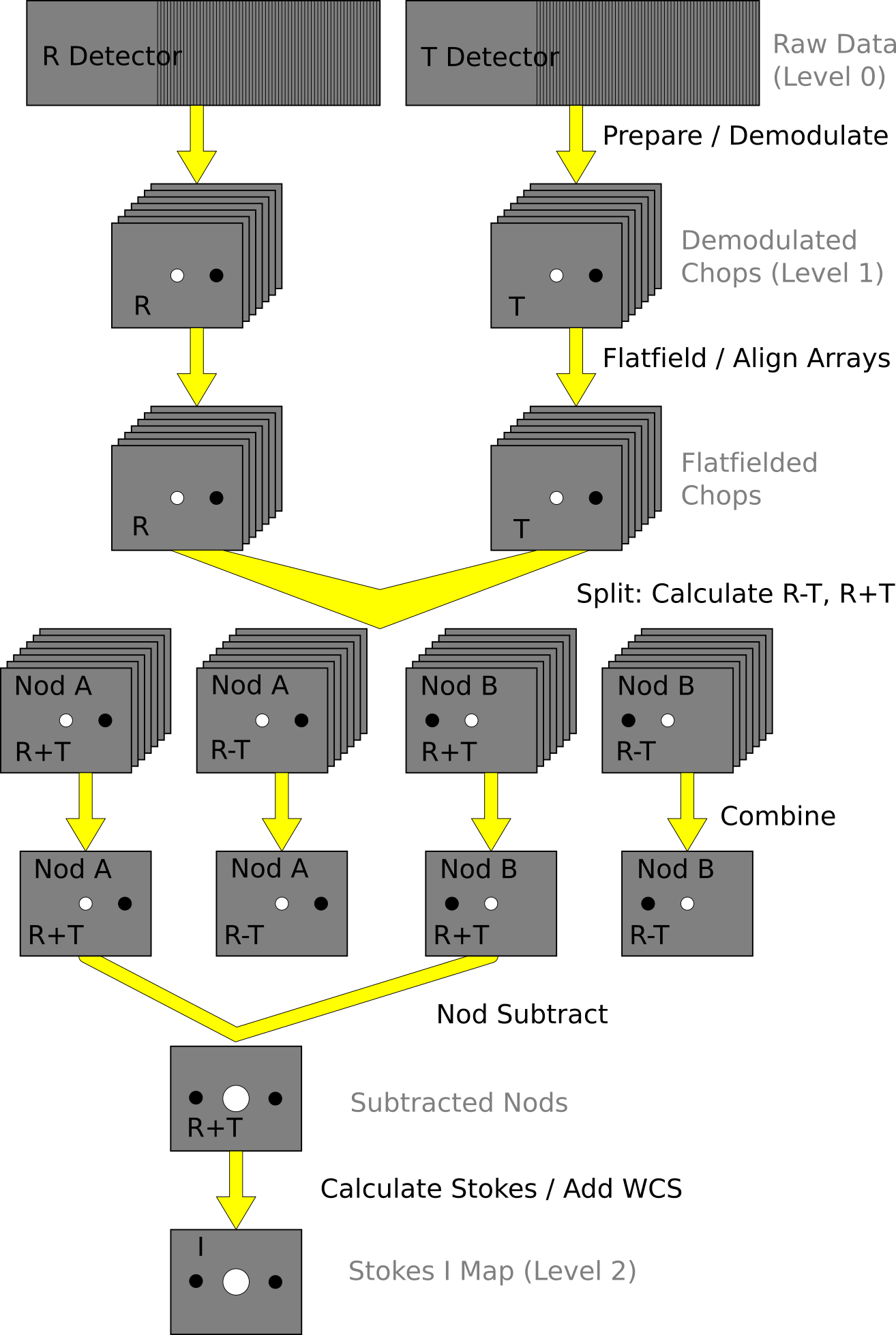
Fig. 102 Chop-Nod data reduction flowchart, up through Stokes parameter calculation for a single input file.

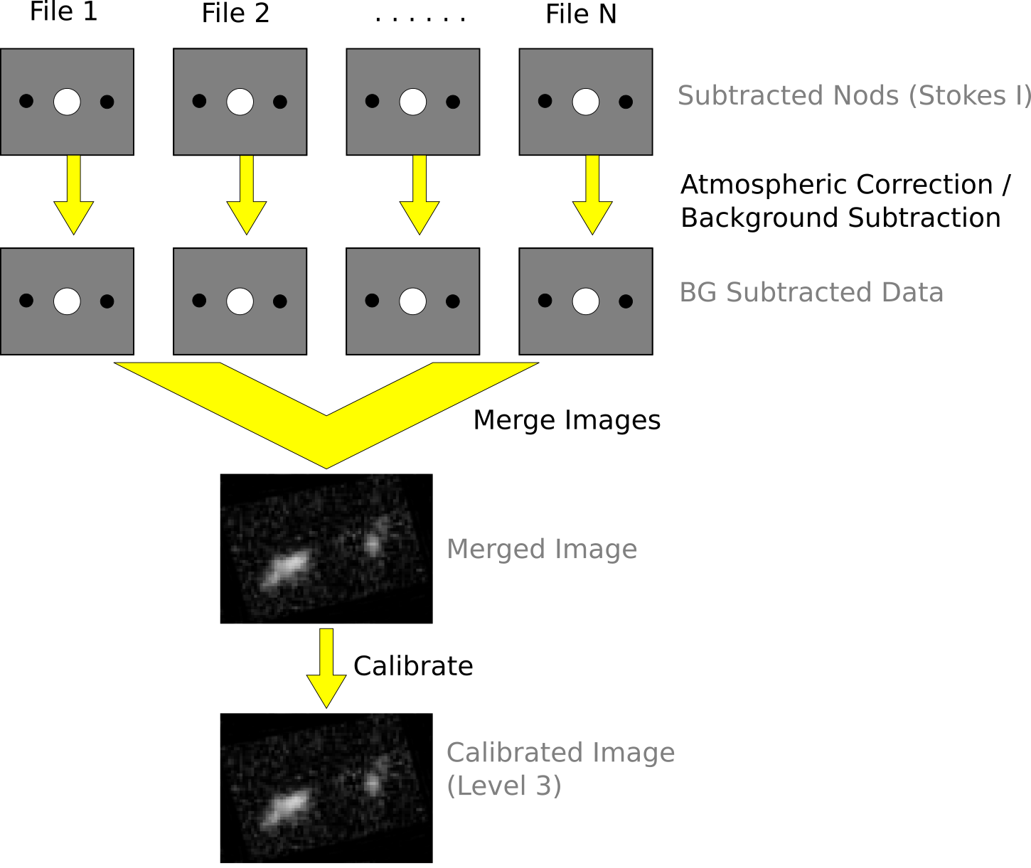
Fig. 103 Chop-Nod data reduction flowchart, picking up from Stokes parameter calculation, through combining multiple input files.

Prepare

The first step in the pipeline is to prepare the raw data for processing, by rearranging and regularizing the raw input data tables, and performing some initial calculations required by subsequent steps.

The raw (Level 0) HAWC files contain all information in FITS binary table extensions located in two Header Data Unit (HDU) extensions. The raw file includes the following HDUs:

• Primary HDU: Contains the necessary FITS keywords in the header but no data. It contains all required keywords for SOFIA data files, plus all keywords required to reduce or characterize the various observing modes. Extra keywords (either from the SOFIA keyword dictionary or otherwise) have been added for human parsing.

• CONFIGURATION HDU (EXTNAME = CONFIGURATION): Contains MCE (detector electronics) configuration data. This HDU is stored only in the raw and demodulated files; it is not stored in Level 2 or higher data products. Nominally, it is the first HDU but users should use EXTNAME to identify the correct HDUs. Note, the “HIERARCH” keyword option and long strings are used in this HDU. All keyword names are prefaced with “MCEn” where n=0,1,2,3. Only the header is used from this HDU.

• TIMESTREAM Data HDU (EXTNAME = TIMESTREAM): Contains a binary table with data from all detectors, with one row for each time sample. The raw detector data is stored in the column “SQ1Feedback”, in FITS (data-store) indices, i.e. 41 rows and 128 columns. Columns 0-31 are for subarray R0, 32-63 for R1, 64-95 for T0 and 96-127 for T1). Additional columns contain other important data and metadata, including time stamps, instrument encoder readings, chopper signals, and astrometry data.

In order to begin processing the data, the pipeline first splits these input TIMESTREAM data arrays into separate R and T tables. It will also compute nod and chop offset values from telescope data, and may also delete, rename, or replace some input columns in order to format them as expected by later algorithms. The output data from this step has the same HDU structure as the input data, but the detector data is now stored in the “R Array” and “T Array” fields, which have 41 rows and 64 columns each.

Demodulate

For both Chop-Nod and Nod-Pol instrument modes, data is taken in a two-point chop cycle. In order to combine the data from the high and low chop positions, the pipeline demodulates the raw time stream with either a square or sine wave-form. Throughout this step, data for each of the R and T arrays are handled separately. The process is equivalent to identifying matched sets of chopped images and subtracting them.

During demodulation, a number of filtering steps are performed to identify good data. By default, the raw data is first filtered with a box high-pass filter with a time constant of one over the chop frequency. Then, any data taken during telescope movement (line-of-sight rewinds, for example, or tracking errors) is flagged for removal. In square wave demodulation, samples are then tagged as being in the high-chop state, low-chop state, or in between (not used). For each complete chop cycle within a single nod position at a single HWP angle, the pipeline computes the average of the signal in the high-chop state and subtracts it from the average of the signal in the low-chop state. Incomplete chop cycles at the end of a nod or HWP position are discarded. The sine-wave demodulation proceeds similarly, except that the data are weighted by a sine wave instead of being considered either purely high or purely low state.

During demodulation, the data is also corrected for the phase delay in the readout of each pixel, relative to the chopper signal. For square wave demodulation, the phase delay time is multiplied by the sample frequency to calculate the delay in data samples for each individual pixel. The data is then shifted by that many samples before demodulating. For sine wave demodulation, the phase delay time is multiplied with 2\(\pi\) times the chop frequency to get the phase shift of the demodulating wave-form in radians.

Alongside the chop-subtracted flux, the pipeline calculates the error on the raw data during demodulation. It does so by taking the mean of all data samples at the same chop phase, nod position, HWP angle, and detector pixel, then calculates the variance of each raw data point with respect to the appropriate mean. The square root of this value gives the standard deviation of the raw flux. The pipeline will propagate these calculated error estimates throughout the rest of the data reduction steps.

The result of the demodulation process is a chop-subtracted, time-averaged flux value and associated variance for each nod position, HWP angle, and detector pixel. The output is stored in a new FITS table, in the extension called DEMODULATED DATA, which replaces the TIMESTREAM data extension. The CONFIGURATION extension is left unmodified.

Flat Correct

After demodulation, the pipeline corrects the data for pixel-to-pixel gain variations by applying a flat field correction. Flat files are generated on the fly from internal calibrator files (CALMODE=INT_CAL), taken before and after each set of science data. Flat files contain normalized gains for the R and T array, so that they are corrected to the same level. Flat files also contain associated variances and a bad pixel mask, with zero values indicating good pixels and any other value indicating a bad pixel. Pixels marked as bad are set to NaN in the gain data. To apply the gain correction and mark bad pixels, the pipeline multiplies the R and T array data by the appropriate flat data. Since the T1 subarray is not available, all pixels in the right half of the T array are marked bad at this stage. The flat variance values are also propagated into the data variance planes.

The output from this step contains FITS images in addition to the data tables. The R array data is stored as an image in the primary HDU; the R array variance, T array data, T array variance, R bad pixel mask, and T bad pixel mask are stored as images in extensions 1 (EXTNAME=”R ARRAY VAR”), 2 (EXTNAME=”T ARRAY”), 3 (EXTNAME=”T ARRAY VAR”), 4 (EXTNAME=”R BAD PIXEL MASK”), and 5 (EXTNAME=”T BAD PIXEL MASK”), respectively. The DEMODULATED DATA table is attached unmodified as extension 6. The R and T data and variance images are 3D cubes, with dimension 64x41xN\(_{frame}\), where N\(_{frame}\) is the number of nod positions in the observation, times the number of HWP positions.

Align Arrays

In order to correctly pair R and T pixels for calculating polarization, and to spatially align all subarrays, the pipeline must reorder the pixels in the raw images. The last row is removed, R1 and T1 subarray images (columns 32-64) are rotated 180 degrees, and then all images are inverted along the y-axis. Small shifts between the R0 and T0 and R1 and T1 subarrays may also be corrected for at this stage. The spatial gap between the 0 and 1 subarrays is also recorded in the ALNGAPX and ALNGAPY FITS header keywords, but is not added to the image; it is accounted for in a later resampling of the image. The output images are 64x40xN\(_{frame}\).

Split Images

To prepare for combining nod positions and calculating Stokes parameters, the pipeline next splits the data into separate images for each nod position at each HWP angle, calculates the sum and difference of the R and T arrays, and merges the R and T array bad pixel masks. The algorithm uses data from the DEMODULATED DATA table to distinguish the high and low nod positions and the HWP angle. At this stage, any pixel for which there is a good pixel in R but not in T, or vice versa, is noted as a “widow pixel.” In the sum image (R+T), each widow pixel’s flux is multiplied by 2 to scale it to the correct total intensity. In the merged bad pixel mask, widow pixels are marked with the value 1 (R only) or 2 (T only), so that later steps may handle them appropriately.

The output from this step contains a large number of FITS extensions: DATA and VAR image extensions for each of R+T and R-T for each HWP angle and nod position, a VAR extension for uncombined R and T arrays at each HWP angle and nod position, as well as a TABLE extension containing the demodulated data for each HWP angle and nod position, and a single merged BAD PIXEL MASK image. For a typical Nod-Pol observation with two nod positions and four HWP angles, there are 8 R+T images, 8 R-T images, 32 variance images, 8 binary tables, and 1 bad pixel mask image, for 57 extensions total, including the primary HDU. The output images, other than the bad pixel mask, are 3D cubes with dimension 64x40xN\(_{chop}\), where N\(_{chop}\) is the number of chop cycles at the given HWP angle.

Combine Images

The pipeline combines all chop cycles at a given nod position and HWP angle by computing a robust mean of all the frames in the R+T and R-T images. The robust mean is computed at each pixel using Chauvenet’s criterion, iteratively rejecting pixels more than 3\(\sigma\) from the mean value, by default. The associated variance values are propagated through the mean, and the square root of the resulting value is stored as an error image in the output.

The output from this step contains the same FITS extensions as in the previous step, with all images now reduced to 2D images with dimensions 64x40, and the variance images for R+T and R-T replaced with ERROR images. For the example above, with two nod positions and four HWP angles, there are still 57 total extensions, including the primary HDU.

Subtract Beams

In this pipeline step, the sky nod positions (B beams) are subtracted from the source nod positions (A beams) at each HWP angle and for each set of R+T and R-T, and the resulting flux is divided by two for normalization. The errors previously calculated in the combine step are propagated accordingly. The output contains extensions for DATA and ERROR images for each set, as well as variance images for R and T arrays, a table of demodulated data for each HWP angle, and the bad pixel mask.

Compute Stokes

From the R+T and R-T data for each HWP angle, the pipeline now computes images corresponding to the Stokes I, Q, and U parameters for each pixel.

Stokes I is computed by averaging the R+T signal over all HWP angles:

\[I = \frac{1}{N} \sum_{\phi=1}^N (R+T)_{\phi},\]

where \(N\) is the number of HWP angles and \((R+T)_{\phi}\) is the summed R+T flux at the HWP angle \(\phi\). The associated uncertainty in I is propagated from the previously calculated errors for R+T:

\[\sigma_I = \frac{1}{N} \sqrt{\sum_{\phi=1}^N \sigma_{R+T,\phi}^2}.\]

In the most common case of four HWP angles at 0, 45, 22.5, and 67.5 degrees, Stokes Q and U are computed as:

\[Q = \frac{1}{2} [(R-T)_{0} - (R-T)_{45}]\]

\[U = \frac{1}{2} [(R-T)_{22.5} - (R-T)_{67.5}]\]

where \((R-T)_{\phi}\) is the differential R-T flux at the HWP angle \(\phi\). Uncertainties in Q and U are propagated from the input error values on R-T:

\[\sigma_Q = \frac{1}{2} \sqrt{\sigma_{R-T,0}^2 + \sigma_{R-T,45}^2}\]

\[\sigma_U = \frac{1}{2} \sqrt{\sigma_{R-T,22.5}^2 + \sigma_{R-T,67.5}^2}.\]

Since Stokes I, Q, and U are derived from the same data samples, they will have non-zero covariance. For later use in error propagation, the pipeline now calculates the covariance between Q and I (\(\sigma_{QI}\)) and U and I (\(\sigma_{UI}\)) from the variance in R and T as follows:

\[\sigma_{QI} = \frac{1}{8} [\sigma_{R,0}^2 - \sigma_{R,45}^2 - \sigma_{T,0}^2 + \sigma_{T,45}^2]\]

\[\sigma_{UI} = \frac{1}{8} [\sigma_{R,22.5}^2 - \sigma_{R,67.5}^2 - \sigma_{T,22.5}^2 + \sigma_{T,67.5}^2]\]

The covariance between Q and U (\(\sigma_{QU}\)) is zero at this stage, since they are derived from data for different HWP angles.

The output from this step contains an extension for the flux and error of each Stokes parameter, as well as the covariance images, bad pixel mask, and a table of the demodulated data, with columns from each of the HWP angles merged. The STOKES I flux image is in the primary HDU. For Nod-Pol data, there will be 10 additional extensions (ERROR I, STOKES Q, ERROR Q, STOKES U, ERROR U, COVAR Q I, COVAR U I, COVAR Q U, BAD PIXEL MASK, TABLE DATA). For Chop-Nod imaging, only Stokes I is calculated, so there are only 3 additional extensions (ERROR I, BAD PIXEL MASK, TABLE DATA).

Update WCS

To associate the pixels in the Stokes parameter image with sky coordinates, the pipeline uses FITS header keywords describing the telescope position to calculate the reference right ascension and declination (CRVAL1/2), the pixel scale (CDELT1/2), and the rotation angle (CROTA2). It may also correct for small shifts in the pixel corresponding to the instrument boresight, depending on the filter used, by modifying the reference pixel (CRPIX1/2). These standard FITS world coordinate system (WCS) keywords are written to the header of the primary HDU.

Subtract Instrumental Polarization

The instrument and the telescope itself may introduce some foreground polarization to the data which must be removed to determine the polarization from the astronomical source. The instrument team uses measurements of the sky to characterize the introduced polarization in reduced Stokes parameters (\(q=Q/I\) and \(u=U/I\)) for each filter band at each pixel. The correction is then applied as

\[Q' = Q - q' I\]

\[U' = U - u' I\]

and propagated to the associated error and covariance images as

\[\sigma_Q' = \sqrt{\sigma_Q^2 + (q' \sigma_I)^2 + 2q'\sigma_{QI}}\]

\[\sigma_U' = \sqrt{\sigma_U^2 + (u' \sigma_I)^2 + 2u'\sigma_{UI}}\]

\[\sigma_{Q'I} = \sigma_{QI} - q' \sigma_I^2\]

\[\sigma_{U'I} = \sigma_{UI} - u' \sigma_I^2\]

\[\sigma_{Q'U'} = -u' \sigma_{QI} - q' \sigma_{UI} + qu\sigma_I^2.\]

The correction is expected to be good to within \(Q/I < 0.6\%\) and \(U/I < 0.6\%\).

Rotate Polarization Coordinates

The Stokes Q and U parameters, as calculated so far, reflect polarization angles measured in detector coordinates. After the foreground polarization is removed, the parameters may then be rotated into sky coordinates. The pipeline calculates a relative rotation angle, \(\alpha\), that accounts for the vertical position angle of the instrument, the initial angle of the half-wave plate position, and an offset position that is different for each HAWC filter. It applies the correction to the Q and U images with a standard rotation matrix, such that:

\[Q' = cos(\alpha) Q + sin(\alpha) U\]

\[U' = sin(\alpha) Q - cos(\alpha) U.\]

The errors and covariances become:

\[\sigma_Q' = \sqrt{(cos(\alpha)\sigma_Q)^2 + (sin(\alpha) \sigma_U)^2 + 2 cos(\alpha) sin(\alpha) \sigma_{QU}}\]

\[\sigma_U' = \sqrt{(sin(\alpha)\sigma_Q)^2 + (cos(\alpha) \sigma_U)^2 - 2 cos(\alpha) sin(\alpha) \sigma_{QU}}\]

\[\sigma_{Q'I} = cos(\alpha) \sigma_{QI} + sin(\alpha) \sigma_{UI}\]

\[\sigma_{U'I} = sin(\alpha) \sigma_{QI} - cos(\alpha) \sigma_{UI}\]

\[\sigma_{Q'U'} = cos(\alpha)sin(\alpha)(\sigma_Q^2 - \sigma_U^2) + (sin^2(\alpha) - cos^2(\alpha)) \sigma_{QU}.\]

Correct for Atmospheric Opacity

In order to combine images taken under differing atmospheric conditions, the pipeline corrects the flux in each individual file for the estimated atmospheric transmission during the observation, based on the altitude and zenith angle at the time when the observation was obtained.

Atmospheric transmission values in each HAWC+ filter have been computed for a range of telescope elevations and observatory altitudes (corresponding to a range of overhead precipitable water vapor values) using the ATRAN atmospheric modeling code, provided to the SOFIA program by Steve Lord. The ratio of the transmission at each altitude and zenith angle, relative to that at the reference altitude (41,000 feet) and reference zenith angle (45 degrees), has been calculated for each filter and fit with a low-order polynomial. The ratio appropriate for the altitude and zenith angle of each observation is calculated from the fit coefficients. The pipeline applies this relative opacity correction factor directly to the flux in the Stokes I, Q, and U images, and propagates it into the corresponding error and covariance images.

Calibrate Flux

The pipeline now converts the flux units from instrumental counts to physical units of Jansky per pixel (Jy/pixel). For each filter band, the instrument team determines a calibration factor in counts/Jy/pixel appropriate to data that has been opacity-corrected to the reference zenith angle and altitude.

The calibration factors are computed in a manner similar to that for another SOFIA instrument (FORCAST), taking into account that HAWC+ is a bolometer, not a photon-counting device. Measured photometry is compared to the theoretical fluxes of objects (standards) whose spectra are assumed to be known. The predicted fluxes in each HAWC+ passband are computed by multiplying the model spectrum by the overall response curve of the telescope and instrument system and integrating over the filter passband. For HAWC+, the standards used to date include Uranus, Neptune, Ceres, and Pallas. The models for Uranus and Neptune were obtained from the Herschel project (see Mueller et al. 2016). Standard thermal models are used for Ceres and Pallas. All models are scaled to match the distances of the objects at the time of the observations. Calibration factors computed from these standards are then corrected by a color correction factor based on the mean and pivot wavelengths of each passband, such that the output flux in the calibrated data product is that of a nominal, flat spectrum source at the mean wavelength for the filter. See the FORCAST GO Handbook, available from the SOFIA webpage, for more details on the calibration process.

Raw calibration factors are computed as above by the pipeline, for any observation marked as a flux standard (OBSTYPE=STANDARD_FLUX), and are stored in the FITS headers of the output data product. The instrument team generally combines these factors across a flight series, to determine a robust average value for each instrument configuration and mode. The overall calibration thus determined is expected to be good to within about 10%.

For science observations, the series-average calibration factor is directly applied to the flux in each of the Stokes I, Q, and U images, and to their associated error and covariance images:

\[I' = I / f\]

\[Q' = Q / f\]

\[U' = U / f\]

\[\sigma_Q' = \sigma_Q / f\]

\[\sigma_U' = \sigma_Q / f\]

\[\sigma_{QI}' = \sigma_{QI} / f^2\]

\[\sigma_{UI}' = \sigma_{UI} / f^2\]

\[\sigma_{QU}' = \sigma_{QU} / f^2.\]

where f is the reference calibration factor. The systematic error on f is not propagated into the error planes, but it is stored in the ERRCALF FITS header keyword. The calibration factor applied is stored in the CALFCTR keyword.

Note that for Chop-Nod imaging data, this factor is applied after the merge step, below.

Subtract Background

After chop and nod subtraction, some residual background noise may remain in the flux images. After flat correction, some residual gain variation may remain as well. To remove these, the pipeline reads in all images in a reduction group, and then iteratively performs the following steps:

• Smooth and combine the input Stokes I, Q, and U images

• Compare each Stokes I image (smoothed) to the combined map to determine any background offset or scaling

• Subtract the offset from the input (unsmoothed) Stokes I images; scale the input Stokes I, Q, and U images

• Compare each smoothed Stokes Q and U images to the combined map to determine any additional background offset

• Subtract the Q and U offsets from the input Q and U images

The final determined offsets (\(a_I, a_Q, a_U\)) and scales (\(b\)) for each file are applied to the flux for each Stokes image as follows:

\[I' = (I - a_I) / b\]

\[Q' = (Q - a_Q) / b\]

\[U' = (U - a_U) / b\]

and are propagated into the associated error and covariance images appropriately.

Rebin Images

In polarimetry, it is sometimes useful to bin several pixels together to increase signal-to-noise, at the cost of decreased resolution. The chop-nod pipeline provides an optional step to perform this binning on individual images, prior to merging them together into a single map.

The Stokes I, Q, and U images are divided into blocks of a specified bin width, then each block is summed over. The summed flux is scaled to account for missing pixels within the block, by the factor:

\[f' = f (n_{pix} / n_{valid})\]

where \(n_{pix}\) is the number of pixels in a block, and \(n_{valid}\) is the number of valid pixels within the block. The error and covariance images are propagated to match. The WCS keywords in the FITS header are also updated to match the new data array.

By default, no binning is performed by the pipeline. The additional processing is generally performed only on request for particular science cases.

Merge Images

All steps up until this point produce an output file for each input file taken at each telescope dither position, without changing the pixelization of the input data. To combine files taken at separate locations into a single map, the pipeline resamples the flux from each onto a common grid, defined such that North is up and East is to the left. First, the WCS from each input file is used to determine the sky location of all the input pixels. Then, for each pixel in the output grid, the algorithm considers all input pixels within a given radius that are not marked as bad pixels. It weights the input pixels by a Gaussian function of their distance from the output grid point and, optionally, their associated errors. The value at the output grid pixel is the weighted average of the input pixels within the considered window. The output grid may subsample the input pixels: by default, there are 4 output pixels for each input pixel. For flux conservation, the output flux is multiplied by the ratio of the output pixel area to the input pixel area.

The error maps output by this algorithm are calculated from the input variances for the pixels involved in each weighted average. That is, the output fluxes from N input pixels are:

\[I' = \frac{\sum_{i}^N w_{i,I} I_i}{w_{tot,I}}\]

\[Q' = \frac{\sum_{i}^N w_{i,Q} Q_i}{w_{tot,Q}}\]

\[U' = \frac{\sum_{i}^N w_{i,U} U_i}{w_{tot,U}}\]

and the output errors and covariances are

\[\sigma_I' = \frac{\sqrt{\sum_{i}^N (w_{i,I} \sigma_{i,I})^2}}{w_{tot,I}}\]

\[\sigma_Q' = \frac{\sqrt{\sum_{i}^N (w_{i,Q} \sigma_{i,Q})^2}}{w_{tot,Q}}\]

\[\sigma_U' = \frac{\sqrt{\sum_{i}^N (w_{i,U} \sigma_{i,U})^2}}{w_{tot,U}}\]

\[\sigma_{QI}' = \frac{\sum_{i}^N w_{i,Q} w_{i,I}\sigma_{i,QI}}{w_{tot,Q}w_{tot,I}}\]

\[\sigma_{UI}' = \frac{\sum_{i}^N w_{i,U} w_{i,I}\sigma_{i,UI}}{w_{tot,U}w_{tot,I}}\]

\[\sigma_{QU}' = \frac{\sum_{i}^N w_{i,Q} w_{i,U}\sigma_{i,QU}}{w_{tot,Q}w_{tot,U}}\]

where \(w_i\) is the pixel weight and \(w_{tot}\) is the sum of the weights of all input pixels.

As of HAWC DRP v2.4.0, the distance-weighted input pixels within the fit radius may optionally be fit by a low-order polynomial surface, rather than a weighted average. In this case, each output pixel value is the value of the local polynomial fit, evaluated at that grid location. Errors and covariances are propagated similarly.

The output from this step is a single FITS file, containing a flux and error image for each of Stokes I, Q, and U, as well as the Stokes covariance images. An image mask is also produced, which represents how many input pixels went into each output pixel. Because of the weighting scheme, the values in this mask are not integers. A data table containing demodulated data merged from all input tables is also attached to the file with extension name MERGED DATA.

Compute Vectors

Using the Stokes I, Q, and U images, the pipeline now computes the polarization percentage (\(p\)) and angle (\(\theta\)) and their associated errors (\(\sigma\)) in the standard way. For the polarization angle \(\theta\) in degrees:

\[\theta = \frac{90}{\pi} arctan\Big(\frac{U}{Q}\Big)\]

\[\sigma_\theta = \frac{90}{\pi (Q^2 + U^2)} \sqrt{(U\sigma_Q)^2 + (Q\sigma_U)^2 - 2 Q U \sigma_{QU}}.\]

The percent polarization (\(p\)) and its error are calculated as

\[p = 100 \sqrt{\Big(\frac{Q}{I}\Big)^2 + \Big(\frac{U}{I}\Big)^2}\]

\[\sigma_p = \frac{100}{I} \sqrt{\frac{1}{(Q^2 + U^2)} \Big[(Q \sigma_Q)^2 + (U \sigma_U)^2 + 2 Q U \sigma_{QU}\Big] + \Big[\Big(\frac{Q}{I}\Big)^2 + \Big(\frac{U}{I}\Big)^2\Big] \sigma_I^2 - 2 \frac{Q}{I}\sigma_{QI} - 2 \frac{U}{I} \sigma_{UI}}.\]

The debiased polarization percentage (\(p'\))is also calculated, as:

\[p' = \sqrt{p^2 - \sigma_p^2}.\]

Each of the \(\theta\), \(p\), and \(p'\) maps and their error images are stored as separate extensions in the output from this step, which is the final output from the pipeline for Nod-Pol data. This file will have 19 extensions, including the primary HDU, with extension names, types, and numbers as follows:

• STOKES I: primary HDU, image, extension 0

• ERROR I: image, extension 1

• STOKES Q: image, extension 2

• ERROR Q: image, extension 3

• STOKES U: image, extension 4

• ERROR U: image, extension 5

• IMAGE MASK: image, extension 6

• PERCENT POL: image, extension 7

• DEBIASED PERCENT POL: image, extension 8

• ERROR PERCENT POL: image, extension 9

• POL ANGLE: image, extension 10

• ROTATED POL ANGLE: image, extension 11

• ERROR POL ANGLE: image, extension 12

• POL FLUX: image, extension 13

• ERROR POL FLUX: image, extension 14

• DEBIASED POL FLUX: image, extension 15

• MERGED DATA: table, extension 16

• POL DATA: table, extension 17

• FINAL POL DATA: table, extension 18

The final two extensions contain table representations of the polarization values for each pixel, as an alternate representation of the \(\theta\), \(p\), and \(p'\) maps. The FINAL POL DATA table (extension 18) is a subset of the POL DATA table (extension 17), with data quality cuts applied.

Scan Reduction Algorithms

This section covers the main algorithms used to reduce Scan mode data. See the flowchart in Fig. 104 for an overview of the iterative process. In this description, “channels” refer to detector pixels, and “frames” refer to time samples read out from the detector pixels during the scan observation.

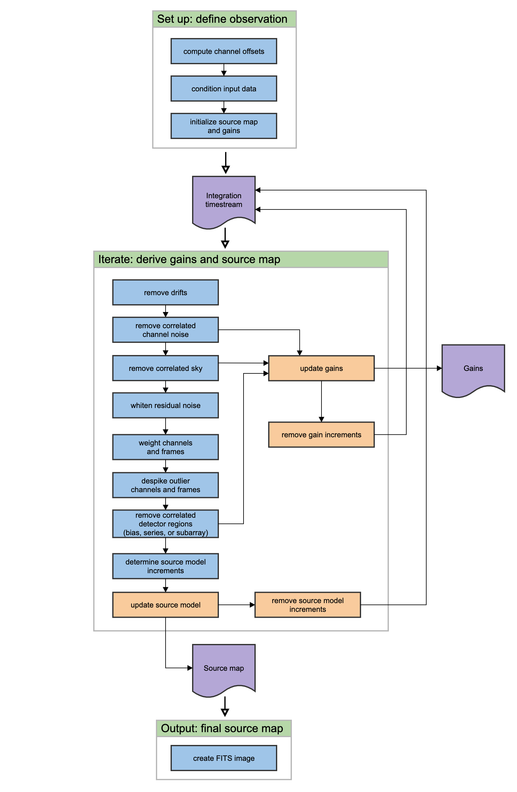
Fig. 104 Scan data reduction flowchart

Signal Structure

Scan map reconstruction is based on the assumption that the measured data (\(X_{ct}\)) for detector \(c\), recorded at time \(t\), is the superposition of various signal components and essential (not necessarily white) noise \(n_{ct}\):

\[X_{ct} = D_{ct} + g_{(1),c} C_{(1),t} + ... + g_{(n),c} C_{(n),t} + G_c M_{ct}^{xy} S_{xy} + n_{ct}\]

We can model the measured detector timestreams via a number of appropriate parameters, such as 1/f drifts (\(D_{ct}\)), \(n\) correlated noise components (\(C_{(1),t} ... C_{(n),t}\)) and channel responses to these (gains, \(g_{(1),c} ... g_{(n),c}\)), and the observed source structure (\(S_{xy}\)). We can derive statistically sound estimates (such as maximum-likelihood or robust estimates) for these parameters based on the measurements themselves. As long as our model is representative of the physical processes that generate the signals, and sufficiently complete, our derived parameters should be able to reproduce the measured data with the precision of the underlying limiting noise.

Below is a summary of the assumed principal model parameters, in general:

• \(X_{ct}\): The raw timestream of channel c, measured at time t.

• \(D_{ct}\): The 1/f drift value of channel c at time t.

• \(g_{(1),c} ... g_{(n),c}\): Channel \(c\) gain (response) to correlated signals (for modes 1 through \(n\)).

• \(C_{(1),t} ... C_{(n),t}\): Correlated signals (for modes 1 through \(n\)) at time \(t\).

• \(G_c\): The point source gain of channel \(c\)

• \(M_{ct}^{xy}\): Scanning pattern, mapping a sky position \(\{x,y\}\) into a sample of channel \(c\) at time \(t\).

• \(S_{xy}\): Actual 2D source flux at position \(\{x,y\}\).

• \(n_{ct}\): Essential limiting noise in channel c at time t.

Sequential Incremental Modeling and Iterations

The pipeline’s approach is to solve for each term separately, and sequentially, rather than trying to do a brute-force matrix inversion in a single step. Sequential modeling works on the assumption that each term can be considered independently from one another. To a large degree this is justified, as many of the signals produce more or less orthogonal imprints in the data (e.g. you cannot easily mistake correlated sky response seen by all channels with a per-channel DC offset). As such, from the point of view of each term, the other terms represent but an increased level of noise. As the terms all take turns in being estimated (usually from bright to faint) this model confusion “noise” goes away, especially with multiple iterations.

Even if the terms are not perfectly orthogonal to one another, and have degenerate flux components, the sequential approach handles this degeneracy naturally. Degenerate fluxes between a pair of terms will tend to end up in the term that is estimated first. Thus, the ordering of the estimation sequence provides a control on handling degeneracies in a simple and intuitive manner.

A practical trick for efficient implementation is to replace the raw timestream with the unmodeled residuals \(X_{ct} \rightarrow R_{ct}\) and let modeling steps produce incremental updates to the model parameters. Every time a model parameter is updated, its incremental imprint is removed from the residual timestream (a process we shall refer to as synchronization).

With each iteration, the incremental changes to the parameters become more insignificant, and the residual will approach the limiting noise of the measurement.

Initialization and Scan Validation

Prior to beginning iterative solution for the model components, the pipeline reads in the raw FITS table, assigns positional offsets to every detector channel, and sky coordinates to every time frame in the scan.

The input timestream is then checked for inconsistencies. For example, HAWC data is prone to discontinuous jumps in flux levels. The pipeline will search the timestream for flux jumps, and flag or fix jump-related artifacts as necessary. The pipeline also checks for gaps in the astrometry data in the timestream, gyro drifts over the course of the observation,

By default, the pipeline also clips extreme scanning velocities using, by default, a set minimum and maximum value for each instrument. The default settings still include a broad range of speeds, so images can sometimes be distorted by low or high speeds causing too little or too much exposure on single pixels. To fix this, the pipeline can optionally remove frames from the beginning or end of the observation, or sigma-clip the telescope speeds to a tighter range.

The size of the output source map is determined from the mapped area on the sky, and a configurable output pixel grid size. This map is updated on each iteration, with the derived source model.

Gains for all detector pixels are initialized with a reference gain map, derived from earlier observations. These initial gains serve as a starting place for the iterative model and allow for flagging and removal of channels known to be bad prior to iterating.

DC Offset and 1/f Drift Removal

For 1/f drifts, consider only the term:

\[R_{ct} \approx \delta D_{c\tau}\]

where \(\delta D_{c\tau}\) is the 1/f channel drift value for \(t\) between \(\tau\) and \(\tau + T\), for a 1/f time window of \(T\) samples. That is, we simply assume that the residuals are dominated by an unmodeled 1/f drift increment \(\delta D_{c\tau}\). Note that detector DC offsets can be treated as a special case with \(\tau = 0\), and \(T\) equal to the number of detector samples in the analysis.

We can construct a \(\chi^2\) measure, as:

\[\chi^2 = \sum_{c,t = \tau}^{t=\tau + T} w_{ct} (R_{ct} - \delta D_{ct})^2\]

where \(w_{ct} = \sigma_{ct}^{-2}\) is the proper noise-weight associated with each datum. The pipeline furthermore assumes that the noise weight of every sample \(w_{ct}\) can be separated into the product of a channel weight \(w_c\) and a time weight \(w_t\), i.e. \(w_{ct} = w_c \cdot w_t\). This assumption is identical to that of separable noise (\(\sigma_{ct} = \sigma_c \cdot \sigma_t\)). Then, by setting the \(\chi^2\) minimizing condition \(\partial \chi^2 / \partial(\delta D_{ct}) = 0\), we arrive at the maximum-likelihood incremental update:

\[\delta D_{c\tau} = \frac{\sum\limits_{t=\tau}^{\tau + T} w_t R_{ct}}{\sum\limits_{t=\tau}^{\tau + T} w_t}\]

Note that each sample (\(R_{ct}\)) contributes a fraction:

\[p_{ct} = w_t / \sum_{t=\tau}^{\tau + T} w_t\]

to the estimate of the single parameter \(\delta D_{c\tau}\). In other words, this is how much that parameter is dependent on each data point. Above all, \(p_{ct}\) is a fair measure of the fractional degrees of freedom lost from each datum, due to modeling of the 1/f drifts. We will use this information later, when estimating proper noise weights.

Note, also, that we may replace the maximum-likelihood estimate for the drift parameter with any other statistically sound estimate (such as a weighted median), and it will not really change the dependence, as we are still measuring the same quantity, from the same data, as with the maximum-likelihood estimate. Therefore, the dependence calculation remains a valid and fair estimate of the degrees of freedom lost, regardless of what statistical estimator is used.

The removal of 1/f drifts must be mirrored in the correlated signals also if gain solutions are to be accurate.

Correlated Noise Removal and Gain Estimation

For the correlated noise (mode \(i\)), we shall consider only the term with the incremental signal parameter update:

\[R_{ct} = g_{(i),c} \delta C_{(i),t} + ...\]

Initially, we can assume \(C_{(i),t}\) as well as \(g_{(i),c} = 1\), if better values of the gain are not independently known at the start. Accordingly, the \(\chi^2\) becomes:

\[\chi^2 = \sum_c w_{ct}(R_{ct} - g_{(i),c} \delta C_{(i),t})^2.\]

Setting the \(\chi^2\) minimizing condition with respect to \(\delta C_{(i),t}\) yields:

\[\delta C_{(i),t} = \frac{\sum\limits_c w_c g_{(i),c} R_{ct}}{\sum\limits_c w_c g_{(i),c}^2}.\]

The dependence of this parameter on \(R_{ct}\) is:

\[p_{ct} = w_c g_{(i),c}^2 / \sum_{c} w_c g_{(i),c}^2\]

After we update \(C_{(i)}\) (the correlated noise model for mode \(i\)) for all frames \(t\), we can update the gain response as well in an analogous way, if desired. This time, consider the residuals due to the unmodeled gain increment:

\[R_{ct} = \delta g_{(i),c} C_{(i),t} + ...\]

and

\[\chi^2 = \sum_t w_{ct}(R_{ct} - \delta g_{(i),c} C_{(i),t})^2\]

Minimizing it with respect to \(\delta g_{(i),c}\) yields:

\[\delta g_{(i),c} = \frac{\sum\limits_t w_t C_{(i),t} R_{ct}}{\sum\limits_t w_t C_{(i),t}^2}\]

which has a parameter dependence:

\[p_{ct} = w_t C_{(i),t}^2 / \sum_{t} w_t C_{(i),t}^2\]

Because the signal \(C_t\) and gain \(g_c\) are a product in our model, scaling \(C_t\) by some factor \(X\), while dividing \(g_c\) by the same factor will leave the product intact. Therefore, our solutions for \(C_t\) and \(g_c\) are not unique. To remove this inherent degeneracy, it is practical to enforce a normalizing condition on the gains, such that the mean gain \(\mu(g_c) = 1\), by construct. The pipeline uses a robust mean measure for gain normalization to produce reasonable comparisons under various pathologies, such as when most gains are zero, or when a few gains are very large compared to the others.

Noise Weighting

Once we model out the dominant signal components, such that the residuals are starting to approach a reasonable level of noise, we can turn our attention to determining proper noise weights. In its simplest form, we can determine the weights based on the mean observed variance of the residuals, normalized by the remaining degrees of freedom in the data:

\[w_c = \eta_c \frac{N_{(t),c} - P_c}{\sum\limits_t w_t R_{ct}^2}\]

where \(N_{(t),c}\) is the number of unflagged data points (time samples) for channel \(c\), and \(P_c\) is the total number of parameters derived from channel \(c\). The scalar value \(\eta_c\) is the overall spectral filter pass correction for channel \(c\), which is 1 if the data was not spectrally filtered, and 0 if the data was maximally filtered (i.e. all information is removed). Thus typical \(\eta_c\) values will range between 0 and 1 for rejection filters, or can be greater than 1 for enhancing filters. We determine time-dependent weights as:

\[w_t = \frac{N_{(c),t} - P_t}{\sum\limits_c w_c R_{ct}^2}\]

Similar to the above, here \(N_{(c),t}\) is the number of unflagged channel samples in frame \(t\), while \(P_t\) is the total number of parameters derived from frame \(t\). Once again, it is practical to enforce a normalizing condition of setting the mean time weight to unity, i.e. \(\mu(w_t) = 1\). This way, the channel weights \(w_c\) have natural physical weight units, corresponding to \(w_c = 1/\sigma_c^2\).

The total number of parameters derived from each channel, and frame, are simply the sum, over all model parameters \(m\), of all the parameter dependencies \(p_{ct}\) we calculated for them. That is,

\[P_c = \sum_m \sum_t p_{(m),ct}\]

and

\[P_t = \sum_m \sum_c p_{(m),ct}\]

Getting these lost-degrees-of-freedom measures right is critical for the stability of the solutions in an iterated framework. Even slight biases in \(p_{ct}\) can grow exponentially with iterations, leading to divergent solutions, which may manifest as over-flagging or as extreme mapping artifacts.

Despiking

After deriving fair noise weights, we can try to identify outliers in the data (glitches and spikes) and flag them for removal from further analysis. By default, the pipeline uses differential deviations between neighboring data points to identify outlier values.

Spectral Conditioning

Ideally, detectors would have featureless white noise spectra (at least after the 1/f noise is treated by the drift removal). In practice, that is rarely the case. Spectral features are bad because (a) they produce mapping features/artifacts (such as “striping”), and because (b) they introduce a covariant noise term between map points that is not easily represented by the output. It is therefore desirable to “whiten” the residual noise whenever possible, to mitigate both these effects.

Noise whitening starts with measuring the effective noise spectrum in a temporal window, significantly shorter than the integration on which it is measured. In the pipeline, the temporal window is designed to match the 1/f stability timescale \(T\) chosen for the drift removal, since the drift removal will wipe out all features on longer timescales. With the use of such a spectral window, we may derive a lower-resolution averaged power-spectrum for each channel. The pipeline then identifies the white noise level, either as the mean (RMS) scalar amplitude over a specified range of frequencies, or automatically, over an appropriate frequency range occupied by the point-source signal as a result of the scanning motion.

Then, the pipeline will look for significant outliers in each spectral bin, above a specified level (and optimally below a critical level too), and create a real-valued spectral filter profile \(\phi_{cf}\) for each channel \(c\) and frequency bin \(f\) to correct these deviations.

There are other filters that can be applied also, such as notch filters, or a motion filter to reject responses synchronous to the dominant telescope motion. In the end, every one of these filters is represented by an appropriate scalar filter profile \(\phi_{cf}\), so the discussion remains unchanged. Only the whitening filter is used by default for HAWC data.

Once a filter profile is determined, we apply the filter by first calculating a rejected signal:

\[\varrho_{ct} = F^{-1}[(1-\phi_{cf}) \hat{R}_{cf}]\]

where \(\hat{R}_{cf}\) is the Fourier transform of \(R_{ct}\), using the weighting function provided by \(w_t\), and \(F^{-1}\) denotes the inverse Fourier Transform from the spectral domain back into the timestream. The rejected signals are removed from the residuals as:

\[R_{ct} \rightarrow R_{ct} - \varrho_{ct}\]

The overall filter pass \(\eta_c\) for channel \(c\), can be calculated as:

\[\eta_c = \frac{\sum\limits_f \phi_{cf}^2}{N_f}\]

where \(N_f\) is the number of spectral bins in the profile \(\phi_{cf}\). The above is simply a measure of the white-noise power fraction retained by the filter, which according to Parseval’s theorem, is the same as the power fraction retained in the timestream, or the scaling of the observed noise variances as a result of filtering.

Map Making

The mapping algorithm for the output source model implements a nearest-pixel method, whereby each data point is mapped entirely into the map pixel that falls nearest to the given detector channel \(c\), at a given time \(t\). Here,

\[\delta S_{xy} = \frac{\sum\limits_{ct} M_{xy}^{ct} w_c w_t \varkappa_c G_c R_{ct}}{\sum\limits_{ct} M_{xy}^{ct} w_c w_t \varkappa_c^2 G_c^2}\]

where \(M_{xy}^{ct}\) associates each sample \(\{c,t\}\) uniquely with a map pixel \(\{x,y\}\), and is effectively the transpose of the mapping function defined earlier. \(\varkappa_c\) is the point-source filtering (pass) fraction of the pipeline. It can be thought of as a single scalar version of the transfer function. Its purpose is to measure how isolated point-source peaks respond to the various reduction steps, and correct for it. When done correctly, point source peaks will always stay perfectly cross-calibrated between different reductions, regardless of what reduction steps were used in each case. More generally, a reasonable quality of cross-calibration (to within 10%) extends to compact and slightly extended sources (typically up to about half of the field-of-view (FoV) in size). While corrections for more extended structures (\(\geq\) FoV) are possible to a certain degree, they come at the price of steeply increasing noise at the larger scales.

The map-making algorithm should skip over any data that is unsuitable for quality map-making (such as too-fast scanning that may smear a source). For formal treatment, we assume that \(M_{ct}^{xy} = 0\) for any troublesome data.

Calculating the precise dependence of each map point \(S_{xy}\) on the timestream data \(R_{ct}\) is computationally costly to the extreme. Instead, the pipeline gets by with the approximation:

\[p_{ct} \approx N_{xy} \cdot \frac{w_t}{\sum\limits_t w_t} \cdot \frac{w_c \varkappa_c^2 G_c}{\sum\limits_c w_c \varkappa_c^2 G_c^2}\]

This approximation is good as long as most map points are covered with a representative collection of pixels, and as long as the pixel sensitivities are more or less uniformly distributed over the field of view.

We can also calculate the flux uncertainty in the map \(\sigma_{xy}\) at each point \(\{x,y\}\) as:

\[\sigma_{xy}^2 = 1 / \sum_{ct} M_{xy}^{ct} w_c w_t \varkappa_c^2 G_c^2\]

Source models are first derived from each input scan separately. These may be despiked and filtered, if necessary, before added to the global increment with an appropriate noise weight (based on the observed map noise) if source weighting is desired.

Once the global increment is complete, we can add it to the prior source model \(S_{xy}^{r(0)}\) and subject it to further conditioning, especially in the intermediate iterations. Conditioning operations may include smoothing, spatial filtering, redundancy flagging, noise or exposure clipping, signal-to-noise blanking, or explicit source masking. Once the model is processed into a finalized \(S_{xy}'\), we synchronize the incremental change \(\delta S_{xy}' = S_{xy}' - S_{xy}^{r(0)}\) to the residuals:

\[R_{ct} \rightarrow R_{ct} - M_{ct}^{xy} (\delta G_c S_{xy}^{r(0)} + G_c \delta S_{xy}')\]

Note, again, that \(\delta S_{xy}' \neq \delta S_{xy}\). That is, the incremental change in the conditioned source model is not the same as the raw increment derived above. Also, since the source gains \(G_c\) may have changed since the last source model update, we must also re-synchronize the prior source model \(S_{xy}^{(0)}\) with the incremental source gain changes \(\delta G_c\) (first term inside the brackets).

The pipeline operates under the assumption that the point-source gains \(G_c\) of the detectors are closely related to the observed sky-noise gains \(g_c\) derived from the correlated noise for all channels. Specifically, it treats the point-source gains as the product:

\[G_c = \varepsilon_c g_c g_s e^{-\tau}\]

where \(\varepsilon_c\) is the point-source coupling efficiency. It measures the ratio of point-source gains to sky-noise gains (or extended source gains). Generally, the pipeline will assume \(\varepsilon_c = 1\), unless these values are measured and loaded during the initial scan validation sequence.

Optionally, the pipeline can also derive \(\varepsilon_c\) from the observed response to a source structure, provided the scan pattern is sufficient to move significant source flux over all detectors. The source gains also include a correction for atmospheric attenuation, for an optical depth \(\tau\), in-band and in the line of sight.

Point-Source Flux Corrections

We mentioned point-source corrections in the section above; here, we explain how these are calculated. First, consider drift removal. Its effect on point source fluxes is a reduction by a factor:

\[\varkappa_{D,c} \approx 1 - \frac{\tau_{pnt}}{T}\]

In terms of the 1/f drift removal time constant \(T\) and the typical point-source crossing time \(\tau_{pnt}\). Clearly, the effect of 1/f drift removal is smaller the faster one scans across the source, and becomes negligible when \(\tau_{pnt} \ll T\).

The effect of correlated-noise removal, over some group of channels of mode \(i\), is a little more complex. It is calculated as:

\[\varkappa_{(i),c} = 1 - \frac{1}{N_{(i),t}} (P_{(i),c} + \sum_k \Omega_{ck} P_{(i),k})\]

where \(\Omega_{ck}\) is the overlap between channels \(c\) and \(k\). That is, \(\Omega_{ck}\) is the fraction of the point source peak measured by channel \(c\) when the source is centered on channel \(k\). \(N_{(i),t}\) is the number of correlated noise-samples that have been derived for the given mode (usually the same as the number of time samples in the analysis). The correlated model’s dependence on channel \(c\) is:

\[P_{(i),c} = \sum_t p_{(i),ct}\]

Finally, the point-source filter correction due to spectral filtering is calculated based on the average point-source spectrum produced by the scanning. Gaussian source profiles with spatial spread \(\sigma_x \approx FWHM / 2.35\) produce a typical temporal spread \(\sigma_t \approx \sigma_x / \bar{v}\), in terms of the mean scanning speed \(\bar{v}\). In frequency space, this translates to a Gaussian frequency spread of \(\sigma_f = (2 \pi \sigma_t)^{-1}\), and thus a point-source frequency profile of:

\[\Psi_f \approx e^{-f^2 / (2\sigma_f^2)}\]

More generally, \(\Psi_f\) may be complex-valued (asymmetric beam). Accordingly, the point-source filter correction due to filtering with \(\phi_f\) is generally:

\[\varkappa_{\phi,c} \approx \frac{\sum\limits_f Re(\phi_f \Psi_f \phi_f)}{\sum\limits_f Re(\Psi_f)}\]

The compound point source filtering effect from \(m\) model components is the product of the individual model corrections, i.e.:

\[\varkappa_c = \prod_m \varkappa_{(m),c}\]

Scan Map Output

Since the Scan mode algorithms are iterative, there are no well-defined intermediate products that may be written to disk. For Scan mode data, the pipeline takes as input a set of raw Level 0 HAWC FITS files, described in the Prepare section, and writes as output a single FITS file per file group, saved with PRODTYPE = scanmap (file name code SMP). These files contain an image of the source map in units of detector counts, and several other extensions.

The flux calibrated map file is saved as the calibrate product type (CAL). The primary HDU in the CAL file contains the flux image in units of Jy/pixel. The first extension (EXTNAME = EXPOSURE) contains an image of the nominal exposure time in seconds at each point in the map. The second extension (EXTNAME = NOISE) holds the error image corresponding to the flux map, and the third extension (EXTNAME = S/N) is the signal-to-noise ratio of the flux to the error image. The fourth and further extensions contain binary tables of data, one for each input scan.

Scan-Pol Reduction Algorithms

Scanning polarimetry reductions are a hybrid of the the Nod-Pol and Scan reduction algorithms, described above.

Scan-Pol observations are performed in a sequence of four scans, where each scan has a different HWP position angle in the following sequence: 5 degrees, 50 degrees, 27.5 degrees, and 72.5 degrees. This sequence is called a ‘set’ hereafter. The pipeline sorts observations into sets and runs the scan map reconstruction algorithm on each set, following the procedure in Scan Reduction Algorithms. For Scan-Pol observations, the pipeline produces two images per scan per HWP angle associated with the R and T arrays. Thus, for a single set, 8 images are generated, one for each of R0 and T0 at each angle. The pipeline creates all maps in the same output coordinate system and pixel scale, so that they are all registered to each other.

Since the scan map step sets the background level independently for each scan image from the median of the full map, there may be inconsistencies in the zero-level between the images, if there is significant diffuse emission across the map. In this case, the pipeline may optionally correct the zero-level in each image by identifying a sky region with no emission, and subtracting the median level in this region from each image. The same region is used for each HWP angle and subarray, so that all images are set independently to a common zero level.

After zero-level correction, the R and T arrays are directly added and subtracted at each HWP angle, and combined as described above to generate Stokes I, Q, and U images (the Compute Stokes step). The output data format is the same as for the stokes product for the Nod-Pol pipeline.

After Stokes calculation, the following steps are also performed, in the way described above for the Nod-Pol pipeline:

• Subtract Instrumental Polarization

• Rotate Polarization Coordinates

• Correct for Atmospheric Opacity

• Merge Images

• Compute Vectors

Note that the scan map pipeline step performs opacity and background level corrections on individual scans and resamples data into sky coordinates with full WCS corrections, as part of its standard processing, so these steps from the Nod-Pol pipeline are not applied.

The final output product is a polarization map, the same as is produced by the Nod-Pol pipeline.

Other Resources

For more information on the code or algorithms used in the HAWC DRP pipeline, see the following documents:

• Far-infrared polarimetry analysis: Hildebrand et. al. 2000 PASP, 112, 1215

• DRP infrastructure and image viewer: Berthoud, M. 2013 ADASS XXII, 475, 193

The scan map reconstruction algorithms are based on a Java pipeline called CRUSH. For more information, see:

• CRUSH paper: Kovács, A. 2008, Proc. SPIE, 7020, 45

• CRUSH thesis: Kovács, A. 2006, PhD Thesis, Caltech

• Online documentation: http://www.sigmyne.com/crush/

Data Products

File names

Output files from the HAWC pipeline are named according to the convention:

FILENAME = F[flight]_HA_[mode]_[aorid]_[spectel]_[type]_[fn1[-fn2]].fits

where flight is the SOFIA flight number, HA indicates the instrument (HAWC+), and mode is either IMA for imaging observations, POL for polarization observations, or CAL for diagnostic data. The aorid indicates the SOFIA program and observation number; spectel indicates the filter/band and the HWP setting. The type is a three-letter identifier for the pipeline product type, and fn1 and fn2 are the first and last raw file numbers that were combined to produce the output product. For example, a polarization map data product with AOR-ID 81_0131_04, derived from files 5 to 6 of flight 295, taken in Band A with HWP in the A position would have the filename F0295_HA_POL_81013104_HAWAHWPA_PMP_005-006.fits. See the tables below for a list of all possible values for the three-letter product type.

Data format

Most HAWC data is stored in FITS files, conforming to the FITS standard (Pence et al. 2010). Each FITS file contains a primary Header Data Unit (HDU) which may contain the most appropriate image data for that particular data reduction level. Most files have additional data stored in HDU image or table extensions. All keywords describing the file are in the header of the primary HDU. Each HDU also has a minimal header and is identified by the EXTNAME header keyword. The algorithm descriptions, above, give more information about the content of each extension.

Pipeline products

The following tables list all intermediate and final products that may be generated by the HAWC pipeline, in the order in which they are produced for each mode. The product type is stored in the primary header, under the keyword PRODTYPE. By default, for Nod-Pol mode, the demodulate, opacity, calibrate, merge, and polmap products are saved. For Chop-Nod mode, the demodulate, opacity, merge, and calibrate products are saved. For Scan mode, the scanmap and calibrate products are saved. For Scan-Pol mode, the scanmappol, calibrate, merge, and polmap products are saved.

For polarization data, the pipeline also generates two auxiliary products: a polarization map image in PNG format, with polarization vectors plotted over the Stokes I image, and a polarization vector file in DS9 region format, for displaying with FITS images. These products are alternate representations of the data in the FINAL POL DATA table in the polarization map (PMP) FITS file. Similarly, for imaging data, a PNG quick-look preview image is generated as a final step in the pipeline. These auxiliary products may be distrubuted to observers separately from the FITS file products.

Data products that contain multiple AORs or that contain observations from multiple flights are referred to as multi-mission products. When multi-mission data are processed and stored in the database, they replace the corresponding single-mission/single-AOR data files. This process usually results in fewer data files for a project. For HAWC+, the following data products can be multi-mission:

• imaging: calibrate (CAL)

• polarimetry: merge (MRG), polmap (PMP).

Table 25 Nod-Pol mode intermediate and final pipeline data products

Step	Description	PRODTYPE	PROCSTAT	Identifier	Saved
Make Flat	Flat generated from Int. Cal file	obsflat	LEVEL_2	OFT	Y
Demodulate	Chops subtracted	demodulate	LEVEL_1	DMD	Y
Flat Correct	Flat field correction applied	flat	LEVEL_2	FLA	N
Align Arrays	R array shifted to T array	shift	LEVEL_2	SFT	N
Split Images	Data split by nod, HWP	split	LEVEL_2	SPL	N
Combine Images	Chop cycles combined	combine	LEVEL_2	CMB	N
Subtract Beams	Nod beams subtracted	nodpolsub	LEVEL_2	NPS	N
Compute Stokes	Stokes parameters calculated	stokes	LEVEL_2	STK	N
Update WCS	WCS added to header	wcs	LEVEL_2	WCS	N
Subtract IP	Instrumental polarization removed	ip	LEVEL_2	IPS	N
Rotate Coordinates	Polarization angle corrected to sky	rotate	LEVEL_2	ROT	N
Correct Opacity	Corrected for atmospheric opacity	opacity	LEVEL_2	OPC	Y
Calibrate Flux	Flux calibrated to physical units	calibrate	LEVEL_3	CAL	Y
Subtract Background	Residual background removed	bgsubtract	LEVEL_3	BGS	N
Bin Pixels	Pixels rebinned to increase S/N	binpixels	LEVEL_3	BIN	N
Merge Images	Dithers merged to a single map	merge	LEVEL_3	MRG	Y
Compute Vectors	Polarization vectors calculated	polmap	LEVEL_4	PMP	Y

Table 26 Chop-Nod mode intermediate and final pipeline data products

Step	Description	PRODTYPE	PROCSTAT	Identifier	Saved
Make Flat	Flat generated from Int.Cal file	obsflat	LEVEL_2	OFT	Y
Demodulate	Chops subtracted	demodulate	LEVEL_1	DMD	Y
Flat Correct	Flat field correction applied	flat	LEVEL_2	FLA	N
Align Arrays	R array shifted to T array	shift	LEVEL_2	SFT	N
Split Images	Data split by nod, HWP	split	LEVEL_2	SPL	N
Combine Images	Chop cycles combined	combine	LEVEL_2	CMB	N
Subtract Beams	Nod beams subtracted	nodpolsub	LEVEL_2	NPS	N
Compute Stokes	Stokes parameters calculated	stokes	LEVEL_2	STK	N
Update WCS	WCS added to header	wcs	LEVEL_2	WCS	N
Correct Opacity	Corrected for atmospheric opacity	opacity	LEVEL_2	OPC	Y
Subtract Background	Residual background removed	bgsubtract	LEVEL_2	BGS	N
Bin Pixels	Pixels rebinned to increase S/N	binpixels	LEVEL_2	BIN	N
Merge Images	Dithers merged to single map	merge	LEVEL_2	MRG	Y
Calibrate Flux	Flux calibrated to physical units	calibrate	LEVEL_3	CAL	Y

Table 27 Scan mode intermediate and final pipeline data products

Step	Description	PRODTYPE	PROCSTAT	Identifier	Saved
Construct Scan Map	Source model iteratively derived	scanmap	LEVEL_2	SMP	Y
Calibrate Flux	Flux calibrated to physical units	calibrate	LEVEL_3	CAL	Y

Table 28 Scan-Pol mode intermediate and final pipeline data products

Step	Description	PRODTYPE	PROCSTAT	Identifier	Saved
Construct Scan Map	Source model iteratively derived	scanmappol	LEVEL_2	SMP	Y
Compute Stokes	Stokes parameters calculated	stokes	LEVEL_2	STK	N
Subtract IP	Instrumental polarization removed	ip	LEVEL_2	IPS	N
Rotate Coordinates	Polarization angle corrected to sky	rotate	LEVEL_2	ROT	N
Calibrate Flux	Flux calibrated to physical units	calibrate	LEVEL_3	CAL	Y
Merge Images	HWP sets merged to single map	merge	LEVEL_3	MRG	Y
Compute Vectors	Polarization vectors calculated	polmap	LEVEL_4	PMP	Y

Grouping Level 0 Data for Processing

In order for the pipeline to successfully reduce a group of HAWC+ data together, all input data must share a common instrument configuration and observation mode, as well as target and filter band and HWP setting. These requirements translate into a set of FITS header keywords that must match in order for a set of data to be grouped together. These keyword requirements are summarized in the table below, for imaging and polarimetry data.

Table 29 Grouping Criteria for Imaging and Polarimetry Modes

Mode	Keyword	Data Type	Match Criterion
All	OBSTYPE	string	exact
All	FILEGPID	string	exact
All	INSTCFG	string	exact
All	INSTMODE	string	exact
All	SPECTEL1	string	exact
All	SPECTEL2	string	exact
All	PLANID	string	exact
All	NHWP	float	exact
Imaging only	SCNPATT	string	exact
Imaging only	CALMODE	string	exact

Configuration and Execution

Installation

The HAWC pipeline is written entirely in Python. The pipeline is platform independent and has been tested on Linux, Mac OS X, and Windows operating systems. Running the pipeline requires a minimum of 16GB RAM, or equivalent-sized swap file.

The pipeline is comprised of six modules within the sofia_redux package: sofia_redux.instruments.hawc, sofia_redux.pipeline, sofia_redux.calibration, sofia_redux.scan, sofia_redux.toolkit, and sofia_redux.visualization. The hawc module provides the data processing algorithms specific to HAWC, with supporting libraries from the calibration, scan, toolkit, and visualization modules. The pipeline module provides interactive and batch interfaces to the pipeline algorithms.

External Requirements

To run the pipeline for any mode from the Redux interface, Python 3.8 or higher is required, as well as the following packages: astropy, astroquery, bottleneck, configobj, cycler, dill, joblib, matplotlib, numba, numpy, pandas, photutils, scikit-learn, and scipy.

Some display functions for the graphical user interface (GUI) additionally require the PyQt5, pyds9, and regions packages. All required external packages are available to install via the pip or conda package managers. See the Anaconda environment file (environment.yml), or the pip requirements file (requirements.txt) distributed with sofia_redux for up-to-date version requirements.

Running the pipeline’s interactive display tools also requires an installation of SAO DS9 for FITS image display. See http://ds9.si.edu/ for download and installation instructions. The ds9 executable must be available in the PATH environment variable for the pyds9 interface to be able to find and control it. Please note that pyds9 is not available on the Windows platform.

Source Code Installation

The source code for the HAWC pipeline maintained by the SOFIA Data Processing Systems (DPS) team can be obtained directly from the DPS, or from the external GitHub repository. This repository contains all needed configuration files, auxiliary files, and Python code to run the pipeline on HAWC data in any observation mode.

After obtaining the source code, install the pipeline with the command:

python setup.py install

from the top-level directory.

Alternately, a development installation may be performed from inside the directory with the command:

pip install -e .

After installation, the top-level pipeline interface commands should be available in the PATH. Typing:

redux

from the command line should launch the GUI interface, and:

redux_pipe -h

should display a brief help message for the command line interface.

Configuration

The DRP pipeline requires a valid and complete configuration file to run. Configuration files are written in plain text, in the INI format readable by the configobj Python library. These files are divided into sections, specified by brackets (e.g. [section]), each of which may contain keyword-value pairs or subsections (e.g. [[subsection]]). The HAWC configuration file must contain the following sections:

• Data configuration, including specifications for input and output file names and formats, and specifications for metadata handling

• Pipeline mode definitions for each supported instrument mode, including the FITS keywords that define the mode and the list of steps to run

• Pipeline step parameter definitions (one section for each pipeline step defined)

The pipeline is usually run with a default configuration file (sofia_redux/instruments/hawc/data/config/pipeconf.cfg), which defines all standard reduction steps and default parameters. It may be overridden with date-specific default values, defined in (sofia_redux/instruments/hawc/data/config/date_overrides/), or with user-defined parameters. Override configuration files may contain any subset of the values in the full configuration file. See Appendix: Sample Configuration Files for examples of override configuration files as well as the full default file.

The scan map reconstruction algorithm, run as a single pipeline step for Scan and Scan-Pol mode data, also has its own separate set of configuration files. These files are stored in the scan module, in sofia_redux/scan/data/configurations. They are read from this sub-directory in the order specified below.

Upon launch, scan map step will invoke the default configuration files (default.cfg) in the following order:

1. Global defaults from sofia_redux/scan/data/config/default.cfg

2. Instrument overrides from sofia_redux/scan/data/config/hawc_plus/default.cfg

Any configuration file may invoke further (nested) configurations, which are located and loaded in the same order as above. For example, hawc_plus/default.cfg invokes sofia/default.cfg first, which contains settings for SOFIA instruments not specific to HAWC.

There are also modified configurations for “faint”, “deep”, or “extended” sources, when one of these flags is set while running the scan map step. For example, the faint mode reduction parses faint.cfg from the above locations, after default.cfg was parsed. Similarly, there are extended.cfg and deep.cfg files specifying modified configurations for extended and deep modes, and a scanpol.cfg file specifying configurations specifically for Scan-Pol mode.

See Appendix: Sample Configuration Files for a full listing of the default configuration for the scan map algorithm.

Input Data

The HAWC pipeline takes as input raw HAWC data files, which contain binary tables of instrument readouts and metadata. The FITS headers contain data acquisition and observation parameters and, combined with the pipeline configuration files and other auxiliary files on disk, comprise the information necessary to complete all steps of the data reduction process. Some critical keywords are required to be present in the raw data in order to perform a successful grouping, reduction, and ingestion into the SOFIA archive. These are defined in the DRP pipeline in a configuration file that describes the allowed values for each keyword, in INI format (see Appendix: Required Header Keywords).

It is assumed that the input data have been successfully grouped before beginning reduction. The pipeline considers all input files in a reduction to be science files that are part of a single homogeneous reduction group, to be reduced together with the same parameters. The sole exception is that internal calibrator files (CALMODE=INT_CAL) may be loaded with their corresponding Chop-Nod or Nod-Pol science files. They will be reduced separately first, in order to produce flat fields used in the science reduction.

Auxiliary Files

In order to complete a standard reduction, the pipeline requires a number of files to be on disk, with locations specified in the DRP configuration file. Current default files described in the default configuration are stored along with the code, typically in the sofia_redux/instruments/hawc/data directory. See below for a table of all commonly used types of auxiliary files.

Table 30 Auxiliary files used by DRP reductions for Chop-Nod and Nod-Pol data

Auxiliary File	File Type	Pipe Step	Comments
Jump Map	FITS	Flux Jump	Contains jump correction values per pixel
Phase	FITS	Demodulate	Contains phase delay in seconds for each pixel
Reference Phase	FITS	Demod. Plots	Contains reference phase angles for comparison with the current observation
Sky Cal	FITS	Make Flat	Contains a master sky flat for use in generating flats from INT_CALs
Flat	FITS	Flat Correct	Contains a back-up flat field, used if INT_CAL files are not available
IP	FITS	Instrumental Polarization	Contains q and u correction factors by pixel and band

The jump map is used in a preparatory step before the pipeline begins processing to correct raw values for a residual electronic effect that results in discontinuous jumps in flux values. It is a FITS image that matches the dimensions of the raw flux values (128 x 41 pixels). Pixels for which flux jump corrections may be required have integer values greater than zero. Pixels for which there are no corrections necessary are zero-valued.

The phase files used in the Demodulate step should be in FITS format, with two HDUs containing phase information for the R and T arrays, respectively. The phases are stored as images that specify the timing delay, in seconds, for each pixel. The reference phase file used in the Demod Plots step is used for diagnostic purposes only: it specifies a baseline set of phase angle values, for use in judging the quality of internal calibrator files.

Normally, the pipeline generates the flat fields used in the Flat Correct step from internal calibrator (INT_CAL) files taken alongside the data. To do so, the Make Flats step uses a Sky Cal reference file, which has four image extensions: R Array Gain, T Array Gain, R Bad Pixel Mask, and T Bad Pixel Mask. The image in each extension should match the dimensions of the R and T arrays in the demodulated data (64 x 41 pixels). The Gain images should contain multiplicative floating-point flat correction factors. The Bad Pixel Mask images should be integer arrays, with value 0 (good), 1 (bad in R array), or 2 (bad in T array). Bad pixels, corresponding to those marked 1 or 2 in the mask extensions, should be set to NaN in the flat images. At a minimum, the primary FITS header for the flat file should contain the SPECTEL1 and SPECTEL2 keywords, for matching the flat filter to the input demodulated files.

When INT_CAL files are not available, the Flat Correct step may use a back-up flat file. This file should have the same format as the Sky Cal file, but the R Array Gain and T Array Gain values should be suitable for direct multiplication with the flux values in the Flat Correct step. There should be one back-up flat file available for each filter passband.

In addition to these files, stored with the DRP code, the pipeline requires several additional auxiliary files to perform flux calibration. These are tracked in the pipecal package, used to support SOFIA flux calibration for several instruments, including HAWC. The required files include response coefficient tables, used to correct for atmospheric opacity, and reference calibration factor tables, used to calibrate to physical units.

The instrumental response coefficients are stored in ASCII text files, with at least four white-space delimited columns as follows: filter wavelength, filter name, response reference value, and fit coefficient constant term. Any remaining columns are further polynomial terms in the response fit. The independent variable in the polynomial fit is indicated by the response filename: if it contains airmass, the independent variable is zenith angle (ZA); if alt, the independent variable is altitude in thousands of feet; if pwv, the independent variable is precipitable water vapor, in \(\mu m\). The reference values for altitude, ZA, and PWV are listed in the headers of the text files, in comment lines preceded with #.

Calibration factors are also stored in ASCII format, and list the correction factor by mode and HAWC filter band, to be applied to opacity-corrected data.

Some additional auxiliary files are used in reductions of flux standards, to assist in deriving the flux calibration factors applied to science observations. These include filter definition tables and standard flux tables, by date and source.

Table 31 Auxiliary files used for calibration (all modes)

Auxiliary File	File Type	Pipe Step	Comments
Response	ASCII	Opacity Correct	Contains instrumental response coefficients by altitude, ZA
Calibration Factor	ASCII	Calibrate	Contains reference calibration factors by filter band, mode
Filter definition	ASCII	Standard Photometry	Contains filter wavelength band and standard aperture definitions
Standard flux	ASCII	Standard Photometry	Contains reference flux values for a known source, by filter band

Automatic Mode Execution

The DPS pipeline infrastructure runs a pipeline on previously-defined reduction groups as a fully-automatic black box. To do so, it creates an input manifest (infiles.txt) that contains relative paths to the input files (one per line). The command-line interface to the pipeline is run as:

redux_pipe infiles.txt

The command-line interface will read in the specified input files, use their headers to determine the observation mode, and accordingly the steps to run and any intermediate files to save. Output files are written to the current directory, from which the pipeline was called. After reduction is complete, the script will generate an output manifest (outfiles.txt) containing the relative paths to all output FITS files generated by the pipeline.

Optionally, in place of a manifest file, file paths to input files may be directly specified on the command line. Input files may be raw FITS files, or may be intermediate products previously produced by the pipeline. For example, this command will complete the reduction for a set of FITS files in the current directory, previously reduced through the calibration step of the pipeline:

redux_pipe *CAL*.fits

To customize batch reductions from the command line, the redux_pipe interface accepts a configuration file on the command line. This file may contain any subset of the full configuration file, specifying any non-default parameters for pipeline steps. An output directory for pipeline products and the terminal log level may also be set on the command line.

The full set of optional command-line parameters accepted by the redux_pipe interface are:

-h, --help            show this help message and exit
-c CONFIG, --configuration CONFIG
                      Path to Redux configuration file.
-o OUTDIR, --out OUTDIR
                      Path to output directory.
-l LOGLEVEL, --loglevel LOGLEVEL
                      Log level.

Manual Mode Execution

In manual mode, the pipeline may be run interactively, via a graphical user interface (GUI) provided by the Redux package. The GUI is launched by the command:

redux

entered at the terminal prompt (Fig. 105). The GUI allows output directory specification, but it may write initial or temporary files to the current directory, so it is recommended to start the interface from a location to which the user has write privileges.

From the command line, the redux interface accepts an optional config file (-c) or log level specification (-l), in the same way the redux_pipe command does. Any pipeline parameters provided to the interface in a configuration file will be used to set default values; they will still be editable from the GUI.

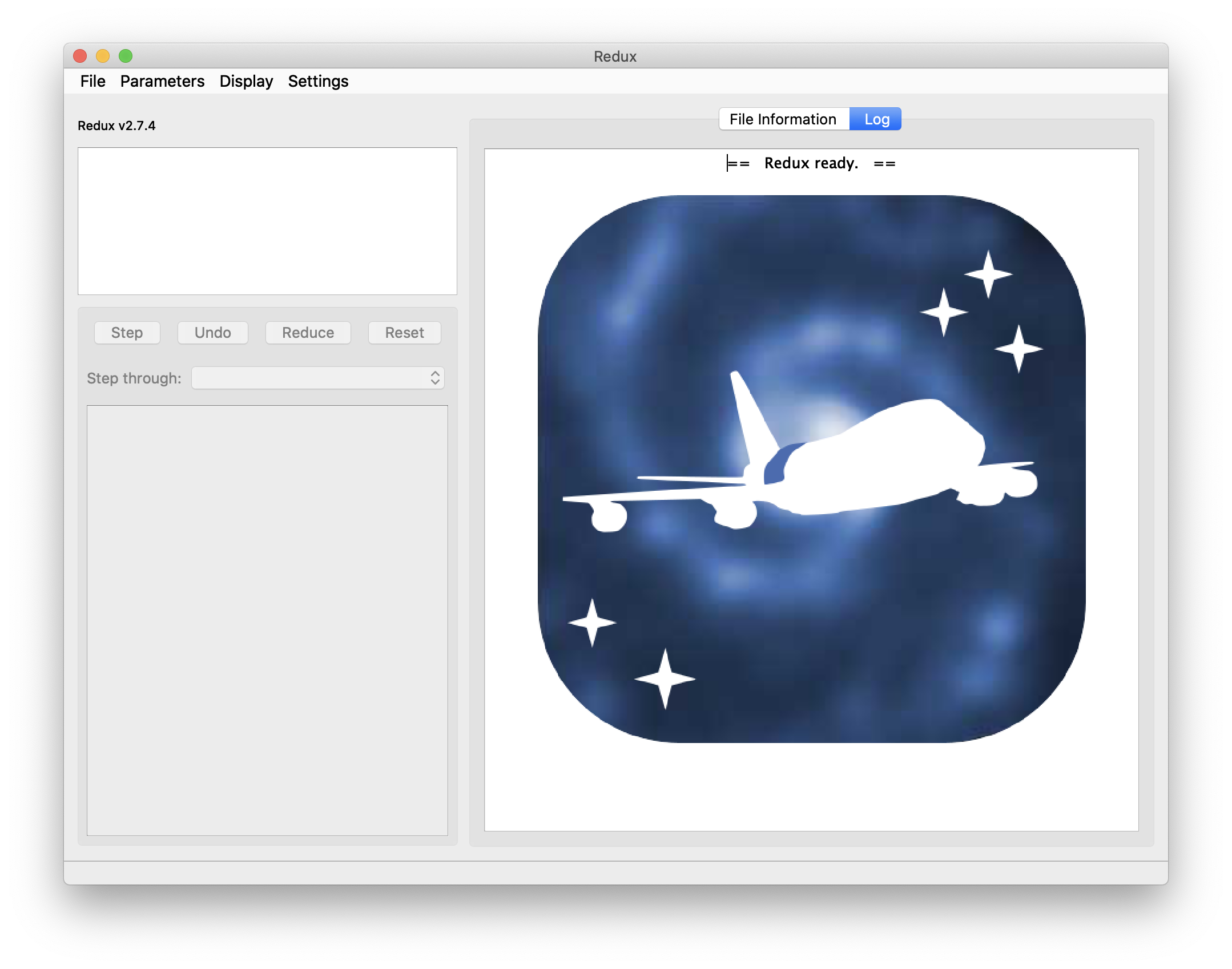
Fig. 105 Redux GUI startup.

Basic Workflow

To start an interactive reduction, select a set of input files, using the File menu (File->Open New Reduction). This will bring up a file dialog window (see Fig. 106). All files selected will be reduced together as a single reduction set.

Redux will decide the appropriate reduction steps from the input files, and load them into the GUI, as in Fig. 107.

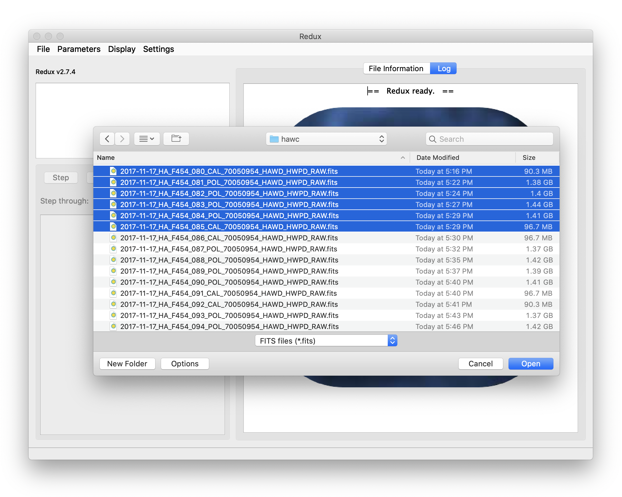
Fig. 106 Open new reduction.

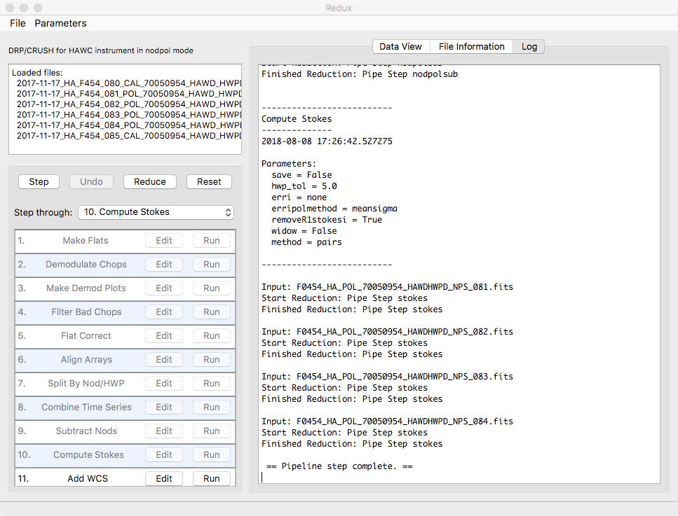
Fig. 107 Sample reduction steps. Log output from the pipeline is displayed in the Log tab.

Each reduction step has a number of parameters that can be edited before running the step. To examine or edit these parameters, click the Edit button next to the step name to bring up the parameter editor for that step (Fig. 108). Within the parameter editor, all values may be edited. Click OK to save the edited values and close the window. Click Reset to restore any edited values to their last saved values. Click Restore Defaults to reset all values to their stored defaults. Click Cancel to discard all changes to the parameters and close the editor window.

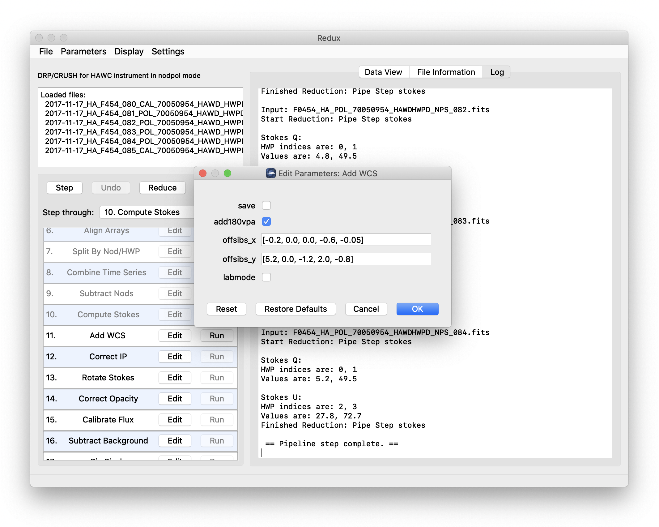
Fig. 108 Sample parameter editor for a pipeline step.

The current set of parameters can be displayed, saved to a file, or reset all at once using the Parameters menu. A previously saved set of parameters can also be restored for use with the current reduction (Parameters -> Load Parameters).

After all parameters for a step have been examined and set to the user’s satisfaction, a processing step can be run on all loaded files either by clicking Step, or the Run button next to the step name. Each processing step must be run in order, but if a processing step is selected in the Step through: widget, then clicking Step will treat all steps up through the selected step as a single step and run them all at once. When a step has been completed, its buttons will be grayed out and inaccessible. It is possible to undo one previous step by clicking Undo. All remaining steps can be run at once by clicking Reduce. After each step, the results of the processing may be displayed in a data viewer. After running a pipeline step or reduction, click Reset to restore the reduction to the initial state, without resetting parameter values.

Files can be added to the reduction set (File -> Add Files) or removed from the reduction set (File -> Remove Files), but either action will reset the reduction for all loaded files. Select the File Information tab to display a table of information about the currently loaded files (Fig. 109).

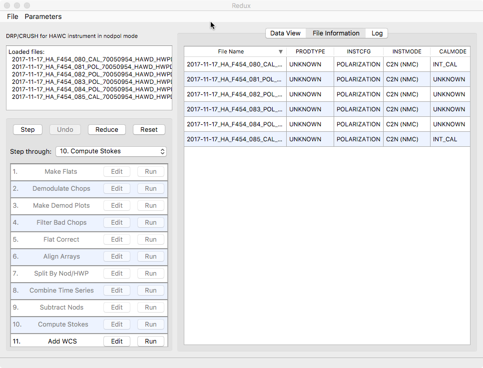
Fig. 109 File information table.

Display Features

The Redux GUI displays images for quality analysis and display (QAD) in the DS9 FITS viewer. DS9 is a standalone image display tool with an extensive feature set. See the SAO DS9 site (http://ds9.si.edu/) for more usage information.

After each pipeline step completes, Redux may load the produced images into DS9. Some display options may be customized directly in DS9; some commonly used options are accessible from the Redux interface, in the Data View tab (Fig. 110).

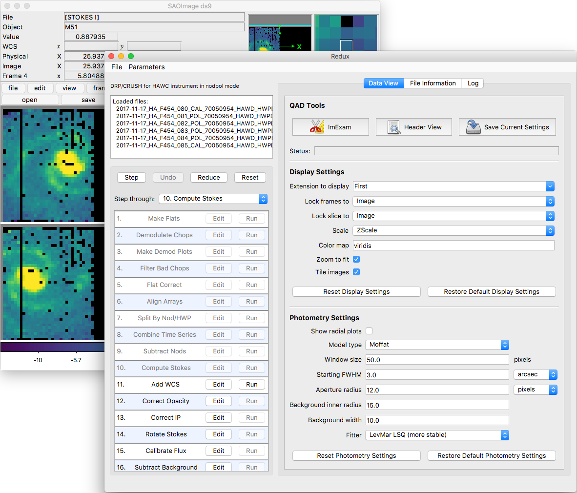
Fig. 110 Data viewer settings and tools.

From the Redux interface, the Display Settings can be used to:

• Set the FITS extension to display (First, or edit to enter a specific extension), or specify that all extensions should be displayed in a cube or in separate frames.

• Lock individual frames together, in image or WCS coordinates.

• Lock cube slices for separate frames together, in image or WCS coordinates.

• Set the image scaling scheme.

• Set a default color map.

• Zoom to fit image after loading.

• Tile image frames, rather than displaying a single frame at a time.

Changing any of these options in the Data View tab will cause the currently displayed data to be reloaded, with the new options. Clicking Reset Display Settings will revert any edited options to the last saved values. Clicking Restore Default Display Settings will revert all options to their default values.

In the QAD Tools section of the Data View tab, there are several additional tools available.

Clicking the ImExam button (scissors icon) launches an event loop in DS9. After launching it, bring the DS9 window forward, then use the keyboard to perform interactive analysis tasks:

• Type ‘a’ over a source in the image to perform photometry at the cursor location.

• Type ‘p’ to plot a pixel-to-pixel comparison of all frames at the cursor location.

• Type ‘s’ to compute statistics and plot a histogram of the data at the cursor location.

• Type ‘c’ to clear any previous photometry results or active plots.

• Type ‘h’ to print a help message.

• Type ‘q’ to quit the ImExam loop.

The photometry settings (the image window considered, the model fit, the aperture sizes, etc.) may be customized in the Photometry Settings. Plot settings (analysis window size, shared plot axes, etc.) may be customized in the Plot Settings. After modifying these settings, they will take effect only for new apertures or plots (use ‘c’ to clear old ones first). As for the display settings, the reset button will revert to the last saved values and the restore button will revert to default values. For the pixel-to-pixel and histogram plots, if the cursor is contained within a previously defined DS9 region (and the regions package is installed), the plot will consider only pixels within the region. Otherwise, a window around the cursor is used to generate the plot data. Setting the window to a blank value in the plot settings will use the entire image.

Clicking the Header button (magnifying glass icon) from the QAD Tools section opens a new window that displays headers from currently loaded FITS files in text form (Fig. 111). The extensions displayed depends on the extension setting selected (in Extension to Display). If a particular extension is selected, only that header will be displayed. If all extensions are selected (either for cube or multi-frame display), all extension headers will be displayed. The buttons at the bottom of the window may be used to find or filter the header text, or generate a table of header keywords. For filter or table display, a comma-separated list of keys may be entered in the text box.

Clicking the Save Current Settings button (disk icon) from the QAD Tools section saves all current display and photometry settings for the current user. This allows the user’s settings to persist across new Redux reductions, and to be loaded when Redux next starts up.

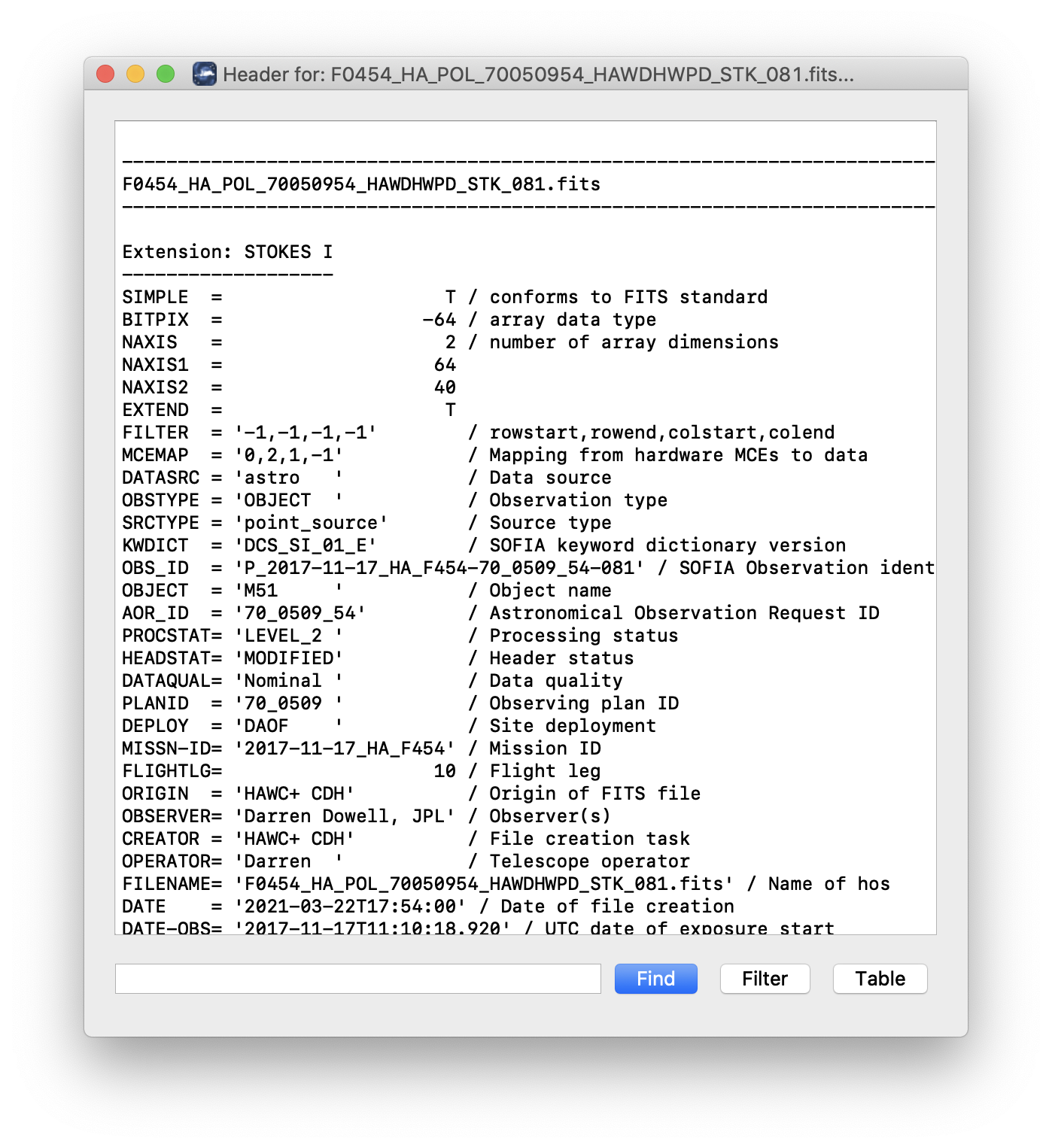
Fig. 111 QAD FITS header viewer.

Important Parameters

Below are some useful parameters for HAWC reductions. Parameters for most pipeline steps may be set directly as key/value pairs in pipeline configuration files; most scan map parameters are added to the options parameter string in pipeline configuration files. All parameters listed are accessible and editable from the Redux GUI interface as well.

The pipeline steps are as named in the configuration file, in the order they are typically run. Not all steps are run for all modes. Note that this list is not exhaustive; see the HAWC+ DRP Developer’s Manual or the code itself for more information.

• checkhead

  • abort: Set to False to allow the pipeline to attempt to continue reduction despite incorrect header keywords. Default is True.

• demodulate

  • phasefile: Set to a FITS file for per-pixel phase shifts, or to a floating point number to apply the same phase shift to all pixels (in seconds of delay). Default is typically a file in hawc/pipeline/data/phasefiles.

  • phaseoffset: Set to a floating point number to apply an offset to the specified phase file. The value should be specified in degrees: it is usually determined from the median offset reported by the demodulation plots for the INT_CAL files. Default is 0.0.

  • track_tol: If non-negative, the pipeline step will use this number as the tracking tolerance in arcseconds. Samples with tracking deviation larger than this number will be rejected. If set to ‘beam’, the beam size for the filter band will be used. If set to ‘centroidexp’, the CentroidExpMsec data stream will be used to flag data, rather than the TrackErrAoi3/4 data stream. Set to -1 to turn off tracking rejection entirely. Default is centroidexp.

  • data_sigma: Sigma threshold for clipping data means; used in calculating variance. Default is 5.0.

• flat

  • flatfile: Set to a file glob to identify flats to use in processing. Default is “flats/*OFT*.fits”.

  • flatfitkeys: Header keywords to match between data and flat fields. Default is “`SPECTEL1’, ‘MISSN-ID’, ‘FILEGPID’, ‘SCRIPTID’”.

  • bkupflat: File glob specifying back-up flats in case flatfile does not exist. Default is “$DPS_HAWCPIPE/pipeline/data/flats/*OFT.fits”.

• split

  • rtarrays: Set to ‘RT’ to use both R and T arrays, ‘R’ for R only, or ‘T’ for T only. Default is ‘RT’.

  • nod_tol: Percent difference between the number of chop cycles in each nod position that will be tolerated for continuing the reduction. Set higher to reject fewer data files. Default is 50.0.

• combine

  • sigma: Reject outliers more than this many sigma from the mean. Default is 3.0.

  • sum_sigma: Reject additional outliers in R+T more than this many sigma from the mean. Default is 4.0.

• scanmap

  • use_frames: Frames (time samples) to use from the reduction. Specify a particular range, as ‘400:-400’ or ‘400:1000’

  • grid: If set, the output pixel size will be modified from the default value to the specified value, in arcsec. The output flux scale will also be modified accordingly, for flux conservation.

  • deep: If set, faint point-like emission is prioritized.

  • faint: If set, faint emission (point-like or extended) is prioritized.

  • extended: If set, extended emission is prioritized. This may increase noise on large angular scales.

  • options: Additional options to pass to the scan map algorithm. Options should be specified by key=value pairs, separated by spaces. For example, ‘rounds=10 sigmaclip=True’. See Appendix: Scan Map Option Glossary for a full list of available options.

• scanmappol

  • save_intermediate: If set, individual output files from the scan map algorithm are saved in separate files. This is primarily for diagnostic use.

  • vpa_tol: If differences between telescope angles (VPA) within a scanpol group are more than this value, this step will issue a warning.

  • use_frames: Frames (time samples) to use from the reduction. Specify a particular range, as ‘400:-400’ or ‘400:1000’

  • grid: If set, the output pixel size will be modified from the default value to the specified value, in arcsec. The output flux scale will also be modified accordingly, for flux conservation.

  • deep: If set, faint point-like emission is prioritized.

  • faint: If set, faint emission (point-like or extended) is prioritized.

  • extended: If set, extended emission is prioritized. This may increase noise on large angular scales.

  • options: Additional options to pass to the scan map algorithm. Options should be specified by key=value pairs, separated by spaces. For example, ‘rounds=10 sigmaclip=True’. See Appendix: Scan Map Option Glossary for a full list of available options.

• stokes

  • erri: Method for inflating errors in I from standard deviation across HWP angles. Can be median, mean, or none. Default is none.

  • removeR1stokesi: Set to False to keep the R1 array in the Stokes I image. Default is True.

• scanstokes

  • zero_level_method: Statistic for zero-level calculation (‘mean’, ‘median’, or ‘none’). If ‘none’, the zero-level will not be corrected. For the other options, either a mean or median statistic will be used to determine the zero-level value from the region set by the region and radius parameters.

  • zero_level_region: If set to ‘header’, the zero-level region will be determined from the ZERO_RA, ZERO_DEC, ZERO_RAD keywords (for RA center, Dec center, and radius, respectively). If set to ‘auto’, a mean- or median-filter will be applied to the R and T images, with the radius specified by the zero_level_radius parameter. The lowest negative local average that is negative in both R and T for all HWP angles is assumed to be the zero level. R and T values are applied separately, from the value of the average at the same pixel. Otherwise, a region may be directly provided as a list of [RA center, Dec center, radius], in degrees.

  • zero_level_radius : Filter radius for zero-level calculation, in arcseconds (per band). Used only for zero_level_region = ‘auto’.

  • zero_level_sigma : Sigma value for statistics clipping. Ignored for zero_level_region = ‘auto’.

• wcs

  • offsibs_x: Offset in pixels along X between SIBS_X and actual target position on array. Should be a comma-separated list of 5 numbers, one for each band; for example, ‘-0.9, 0.0, 1.1, 0.0, 1.1’. Default may vary over time.

  • offsibs_y: Offset in pixels along Y between SIBS_Y and actual target position on array, as for offsibs_x. Default may vary over time.

• ip

  • qinst: Fractional instrumental polarization in q. Should be a comma-separated list of 5 numbers, one for each band; for example, ‘-0.01191, 0.0, -0.01787, -0.00055, -0.01057’. Default may vary over time.

  • uinst: Fractional instrumental polarization in u, as for qinst.

  • fileip: FITS file specifying IP corrections for each pixel and band. If set to ‘uniform’, the step will use the qinst and uinst values; otherwise, these values are ignored if fileip is specified.

• rotate

  • gridangle: Detector angle offset, in degrees. Should be a comma-separated list of 5 numbers, one for each band; for example, ‘-89.69, 0.0, -104.28, 37.42, 119.62’. Default may vary over time.

• bgsubtract

  • bgslope: Number of iterations to run with slope term. If zero, slope will not be fit (i.e. residual gains will not be corrected). Default is 0.

  • bgoffset: Number of iterations to run with offset term. If zero, offset will not be fit (i.e. residual background will not be removed). Default is 10.

  • qubgsubtract: Set to True to calculate and remove offsets in Q and U maps, in addition to Stokes I. Default is True; must be set to False for Chop-Nod data.

• binpixels

  • block_size: Bin size, in pixels. The value provided must divide the 64x40 array evenly into square blocks. Values 2, 4, or 8 will work. If set to 1, no binning will be performed. Default value is 1.

• merge

  • cdelt: Pixel size in arcseconds of output map, one number per band. Decrease to sub-sample the input pixels more. Default is ‘1.21, 1.95, 1.95, 3.40, 4.55’, half the detector pixel scale (beam size / 4).

  • fwhm: FWHM in arcseconds of Gaussian smoothing kernel, by band. Make larger for more smoothing. Default is ‘4.84, 7.80, 7.80, 13.6, 18.2’, for beam-size smoothing.

  • radius: Integration radius for input pixels, by band. Set larger to consider more pixels when calculating output map. Default is ‘9.68, 15.6, 15.6, 27.2, 36.4’ (beam-size * 2).

  • fit_order: Polynomial fit order for local regression. Default is 2.

  • errflag: Set to True to use error image for weighting. Default is True.

  • edge_threshold: Threshold to set edge pixels to NaN. Range is 0-1; 0 means keep all edge pixels. Higher values keep fewer pixels.

  • adaptive_algorithm: If ‘shaped’ or ‘scaled’, adaptive smoothing will be used, varying the kernel size according to the data. If ‘shaped’, the kernel shape and rotation angle may also vary. Set to ‘none’ to turn off adaptive smoothing.

  • fit_threshold: Deviation from weighted mean to allow for higher order fit. Set to 0 to turn off. Positive values replace bad values with the mean value in the window; negative values replace bad values with NaN.

  • bin_cdelt: If set, and data was previously binned via the binpixels step, then the input cdelt and radius will be multiplied by the binning factor. If not set, the provided cdelt will be used directly. This allows useful default behavior for binned data, but still allows for tunable output pixel sizes.

• region

  • skip: Set to a number \(i\) to keep vectors every \(i\)th pixel. Default is 2 (as appropriate for cdelt=beamsize/4 in merge step).

  • mini: Do not keep vectors from pixels with Stokes I flux less than this fraction of peak flux. Default is 0.0.

  • minisigi: Do not keep vectors from pixels with Stokes I flux less than this many sigma. Default is 200.

  • minp: Do not keep vectors with percent polarization less than this value. Default is 0%.

  • maxp: Do not keep vectors with percent polarization greater than this value. Default is 50%.

  • sigma: Do not keep vectors with \(p / \sigma_p\) less than this value. Default is 3.0.

  • length: Scale factor for polarization vectors in DS9 region file, in pixels. Default is 10 (i.e. a 10% polarization vector is the length of one pixel).

  • rotate: Plot rotated (B field) vectors in DS9 region file. Default is True.

  • debias: Plot debiased vectors in DS9 region file. Default is True.

• polmap

  • maphdu: Extension to use for the plot. Default is ‘STOKES I’.

  • lowhighscale: [low, high] percentile values to use for image scaling. Default is 0.25,99.75.

  • scalevec: Scale factor for polarization vectors in polmap image. Default is 0.0003.

  • scale: If True, plotted vectors are scaled by their magnitude. If False, all vectors are plotted at the same length. Default is True.

  • rotate: Plot rotated (B field) vectors in polmap image. Default is True.

  • debias: Use debiased polarizations for plotting. Default is True.

  • colorvec: Color to use for vectors in polmap image. Default is ‘black’.

  • colormap: Color map to use in polmap image. Default is ‘plasma’. Any valid Matplotlib color map name may be specified.

  • ncontours: Number of contour levels. Set to 0 to turn off contours. Default is 30.

  • colorcontour: Color to use for contour lines in polmap image. Default is ‘gray’.

  • fillcontours: If True, contours are filled. Default is True.

  • grid: If True, a coordinate grid is overlaid. Default is True.

  • title: Title for the plot. If set to ‘info’, the title is auto-generated from the FITS file information. Any other string will be used directly as the title. Default is ‘info’.

  • centercrop: If True, the plot is cropped to the dimensions specified in the centercropparams. Default is False.

  • centercropparams: Specifies the crop region if centercrop = True. Should be specified as [RA, Dec, width, height] in decimal degrees.

  • watermark: If set to a non-empty string, the text will be added to the lower-right of the image as a semi-transparent watermark.

• imgmap

  • maphdu: Extension to use for the plot. Default is ‘STOKES I’.

  • lowhighscale: [low, high] percentile values to use for image scaling. Default is 0.25,99.75.

  • colormap: Color map to use in polmap image. Default is ‘plasma’. Any valid Matplotlib color map name may be specified.

  • ncontours: Number of contour levels. Set to 0 to turn off contours. Default is 0.

  • colorcontour: Color to use for contour lines in polmap image. Default is ‘gray’.

  • fillcontours: If True, contours are filled. Default is True.

  • grid: If True, a coordinate grid is overlaid. Default is False.

  • title: Title for the plot. If set to ‘info’, the title is auto-generated from the FITS file information. Any other string will be used directly as the title. Default is ‘info’.

  • centercrop: If True, the plot is cropped to the dimensions specified in the centercropparams. Default is False.

  • centercropparams: Specifies the crop region if centercrop = True. Should be specified as [RA, Dec, width, height] in decimal degrees.

  • watermark: If set to a non-empty string, the text will be added to the lower-right of the image as a semi-transparent watermark.

Data Quality Assessment

After the pipeline has been run on a set of input data, the output products should be checked to ensure that the data has been properly reduced. Data quality and quirks can vary widely across individual observations, but the following general guideline gives some strategies for approaching quality assessment for HAWC+ data.

For any mode:

• Check the instrument scientist’s log for any data that is known to be of poor or questionable quality.

• Check the output to the log file (usually called redux_[date]_[time].log), written to the same directory as the output files. Look for messages marked ERROR or WARNING. The log will also list every parameter used in DRP steps, which may help disambiguate the parameters as actually-run for the pipeline.

• Check that the expected files were written to disk. There should be, at a minimum, a DMD, WCS, CAL, and PMP file for Nod-Pol data, and a CRH and CAL file for Scan data.

For Nod-Pol or Scan-Pol mode:

• Display all CAL files together. Verify that no one file looks unreasonably noisy compared to the others, and that any visible sources appear in the same locations, according to the world coordinate system in each file’s header. Particular CAL files may need to be excluded, and the last steps of the pipeline re-run.

• Check the CAL files for persistent bad pixels or detector features. If present, the flat field or bad pixel mask may need updating.

• Display the final PMP file. Verify that the mapping completed accurately, with no unexpected or unusual artifacts. The weighting flags may need modification, or the smoothing may need to be increased.

• Overlay the DS9 polarization vector file (*.reg) on the PMP file. Check for unusually noisy vector maps (e.g. long vectors near the edges).

• For observations of flux standards, compare the total flux in the source, via aperture photometry, to a known model. Flux calibration should be within 20%; if it is not, the calibration factors may need to be adjusted, or some off-nominal data may need to be excluded from the reduction.

• For observations of polarimetric standards, verify that the total polarization (Q/I and U/I) is less than 0.6% in regions that should have zero total polarization. If it is not, the instrumental polarization parameters may need adjusting.

• Check that sources appear at the expected coordinates. If they do not, the boresight offsets used by the pipeline may need to be adjusted.

• Check the FHWM and PSF shape of the source. If it is larger than expected, or not round, there may have been a problem with telescope guiding or chopping/nodding.

• If there are output products from the chi2 pipeline, review them for discrepancies between sets of dithers, or excessive noise or artifacts.

For Scan or Scan-Pol mode:

• Check the log for warnings about scans that may have been excluded from reduction or are of poor quality.

• Display the final CRH image. Check that no unusual artifacts appear (e.g. holes or “worms” caused by bad pixels that were not properly excluded from the scans). Try reducing the data with the -fixjumps option to see if these artifacts improve.

• Check that the map is not unusually large and does not include patches disconnected from the main image. These may be signs of poor tracking during the observation or missing metadata in the input FITS tables. Try reducing each scan individually to see if a bad scan may be identified and excluded.

• For observations of flux standards, compare the total flux in the source, via aperture photometry, to a known model. Flux calibration should be within 20%; if it is not, the calibration factors or the opacity correction may need to be adjusted.

• Check the FHWM and PSF shape of the source. If it is larger than expected, or not round, there may have been a problem with telescope guiding or focus.

• Check that the source is at the expected coordinates. If not, the boresight offsets may need to be adjusted. Check the SIBSDX and SIBSDY keywords in the header.

• If the target is not visible in the default reduction, try reducing the data with the faint option. Note: this option should be used for scan mode only; it should not be used for Scan-Pol observations.

• If the target has extended diffuse emission, it may be beneficial to try reducing the data with the extended option. If applied to Scan-Pol observations, compare the polarization maps from the regular pipeline and the output from the extended parameter. Check for inconsistent vectors in the polarization map. If not sure of the output, contact the lead Instrument Scientist for feedback.

Appendix: Scan Map Option Glossary

Table 32 Configuration Keywords

Keyword	Usage in configuration file	Description
1overf.freq	[1overf] freq=<X>	The target frequency X (Hz) at which the 1/f is measured for logging global 1/f noise statistics. The logged quantity is the ratio of the PSD measured at this frequency to that measured at the reference frequency 1overf.ref. The actual measurement frequency will always be above the filter cutoff of drifts filtering.
1overf.ref	[1overf] ref=<X>	The white noise reference frequency X (Hz) used when providing 1/f noise statistics. If the value exceeds the Nyquist frequency of the timestream, then the Nyquist value will be used instead. See 1overf.freq.
accel Alias: correlated.accel-mag	[accel] <options…>	Can be used to enable acceleration response decorrelation, or to set options for it. See correlated.<modality> for available options.
aclip	aclip=<X>	Clip data when the telescope acceleration is above X arcsec/s^2. Heavy accelerations can put mechanical energy into the detector system, changing the shape of the primary, thereby generating bright signals from the varying illumination of the bright atmosphere. Clipping data when there is danger of this happening is a good idea. See accel for possible modelling of these signals.
add	add={<key>, <key>=<value>}, …	Add a key to the configuration. If only <key> is given, it’s value will be set to ‘True’. Multiple keys and values may be added to the configuration by supplying a comma-separated list.
aliases	[aliases] <branch1>=<alias1> <branch2>=<alias2> …	The [aliases] section specifies user defined convenient shorthand notations for configuration keywords. For example, if one defines the alias sky=correlated.sky, then sky.gainrange will actually reference correlated.sky.gainrange for any configuration operation. Aliases may also reference other aliases, so sg=sky.gainrange would allow sg to reference correlated.sky.gainrange.
altaz Sets: system=horizontal	altaz={True, False}	A conditional switch to reduce in Alt/Az coordinates. See system.
array Alias for: correlated.obs-channels	[array] <options…>	An alias for all radiation-sensitive channels of the instrument, or set options for it. See correlated.<modality> for further details.
atran.altcoeffs Instrument: SOFIA	atran.altcoeffs=<c0>,<c1>,<c2>,…<cN>	The polynomial coefficients used to determine the altitude factor when determining the atmospheric transmission correction. Used to fit for an altitude relative to 41 kft in units of kft.
atran.amcoeffs Instrument: SOFIA	atran.amcoeffs=<c0>,<c1>,<c2>,…<cN>	The polynomial coefficients used to determine the air mass factor when determining the atmospheric transmission correction. Used to fit for the air mass relative to sqrt(2) (an elevation of 45 degrees).
atran.reference Instrument: SOFIA	atran.reference=<X>	The factor (f) used to provide the actual transmission value when multiplied by the transmission correction value (c). The transmission (t) is given as t = f * c where c = am_factor * alt_factor (see atran.altcoeffs and atran.amcoeffs). The transmission is related to the opacity (tau) by t = exp(-tau * airmass).
beam	beam=<X>	Set the instrument beam to X arcseconds. Also see resolution.
beammap Sets: pixelmap=True	beammap={True, False}	A conditional switch that sets pixelmap to True.
blacklist	blacklist=<key1>,<key2>,…	Similar to forget, except it will not set options even if they are specified at a later time. This is useful for altogether removing settings from the configuration.
blank	blank=<X>	Skip data from modelling over points that have a source flux exceeding the signal-to-noise level X. This may be useful in reducing the filtering effect around bright See clip.
blind	blind=<range list>	Specify a list of blind pixels. Use data indices and ranges in a comma-separated form. Blind channels may be used by some instruments to estimate instrumental signals, such as temperature fluctuations. Channels are numbered from 0 (C-style). See flag. <range list> is a comma-separated list of individual channels or channel ranges. For example: blind=10,15:18,33 Would blind channels 10, 15, 16, 17, 18, and 33.
bright Sets: config=bright.cfg	bright={True, False}	Use for bright sources (S/N > ~1000). This setting entirely bypasses all filtering to produce a very faithful map. The drawback is more noise. See config, faint, and deep.
chopped	chopped={True, False}	Used for specifying a chopped data reduction. Can be set manually or automatically based on the data itself. The key may trigger conditional statements and extra decorrelation steps. See correlated.<modality>.trigger.
chopper.invert Instrument: HAWC+	chopper.invert={True, False}	An option to flip the direction associated with the analog chopper R/S signals.
chopper.shift Instrument: HAWC+	chopper.shift=<N>	Shift the chopper R/S analog signals by N raw frames (sampled at 203.25 Hz), relative to the detector readout to improve synchronization. See shift.
chopper.tolerance Instrument: HAWC+	chopper.tolerance=<X>	Allow setting a tolerance for the chopper position in arcseconds. If the actual chopper distance is not within the tolerance from the nominal chopper amplitude, then the exposure will not be used to avoid smearing.
clip	clip=<X>	In early generations of the source map, force map pixels with flux below signal-to-noise level X to zero. This may help getting lesser baselines, and filtering artifacts around the brighter peaks. Often used together with blank in the intermediate iterations. See blank and iteration.
cols Alias: correlated.cols	[cols] <options…>	An alias for column based decorrelation of the detector array. Used to perform decorrelation, or set decorrelation options.
commonwcs	commonwcs={True, False}	If the reduction consists of multiple sub-reductions (e.g. a sub reduction for each HAWC+ subarray), specify that the output map for all reductions should share a common WCS and equivalent dimensions.
conditionals	[conditionals] [[<requirement>]] <key1>=<value1> …	Used to set configuration values in specific circumstances. Multiple key=value settings can be applied under each requirement once that requirement has been fulfilled. Requirements should take the form [[<keyword>]] or [[<keyword><operator><value>]]. The first will apply settings should that keyword be set in the configuration. The more complex alternative involves comparing one configuration keyword value with another in the requirement, and apply all settings if evaluated as true. <operator> can be one of =, !=, <, <=, >, or >=.
config	config=<filename>	Load a configuration file filename. Files are looked for in the following order from lowest to highest priority in the sofia_scan/scan/data/configurations folder (<c>) and a optional user configuration directory (~/.sofscan): <c>/<filename> ~/.sofscan/<filename> <c>/<instrument>/<filename> ~/.sofscan/<instrument>/<filename> Whenever a matching file is found, its contents are parsed. Because of the ordering, it is convenient to create overriding configurations. Each successively loaded file may override the options set before it. See bright, faint, and deep.
correlated.<modality>	[correlated] [[<modality>]] <key>=<value> …	Remove the correlated noise term across the entire array where <modality> is the name of the modality on which decorrelation is performed. E.g. ‘obs-channels’ or ‘gradients’. This is an effective way of dealing with most atmospheric and instrumental signals, such as sky noise, ground pickup, temperature fluctuations, electromagnetic or microphonic pickups. The decorrelation of each modality can be further controlled by a number of <key>=<value> settings (see below). The given decorrelation step must also appear in the pipeline ordering before it can be used. See division.<name> and ordering.
correlated.<modality>. gainrange	[correlated] [[<modality>]] gainrange=<min>:<max>	Specify a range of acceptable gains to the given correlated signal <modality>, relative to the average gain response of the correlated mode. Channels that exhibit responses outside of this range will be appropriately flagged in the reduction, and ignored in the modelling steps until the flag is revised and cleared in another decorrelation step. See division.<name>.gainflag and correlated.<modality>.signed.
correlated.<modality>. nofield	[correlated] [[<modality>]] nofield={True, False}	Allow decoupling of the gains of the correlated mode from the gain fields stored under the channel (initialized from the file specified by pixeldata). See pixeldata and source.fixedgains.
correlated.<modality>. nogains	[correlated] [[<modality>]] nogains={True, False}	Disable the solving of gains (i.e. channel responses) to the correlated signal <modality>.
correlated.<modality>. nosignals	[correlated] [[<modality>]] nosignals={True, False}	Disable solving for the correlated signal <modality> whose value stays fixed.
correlated.<modality>. phases	[correlated] [[<modality>]] phases={True, False}	Decorrelate the phase data (e.g. for chopped photometry scans) together with the fast samples. The same gains are used as for the usual decorrelation on the fast samples.
correlated.<modality>. phasegains	[correlated] [[<modality>]] phasegains={True, False}	Determine the gains from the phase data, rather than from the correlated fast samples. You can also set this globally for all correlated modalities/modes using the phasegains keyword. See phasegains.
correlated.<modality>. resolution	[correlated] [[<modality>]] resolution=<X>	Set the time resolution (in seconds) for the decorrelation of <modality>. When dealing with 1/f-type signals, you probably want to set this to the 1/f knee time-scale or below if you want optimal sensitivities. Else, you may want to try larger values if you want to recover more large-scale emission and are not too worried about the loss of sensitivity. See extended.
correlated.<modality>. signed	[correlated] [[<modality>]] signed={True, False}	by default, gain responses are allowed to be bidirectional, and flagging affects only those channels or pixels, where absolute gain values fall outside of the specified range. When ‘signed’ is set, the gains are flagged with the signs also taken into account. I.e., under ‘signed’, ‘gainrange’ or ‘0.3:3.0’ would flag pixels with a gain of -0.8, whereas the default behaviour is to tolerate them. See correlated.<modality>.gainrange and correlated.<modality>.nogains.
correlated.<modality>. span	[correlated] [[<modality>]] span={True, False}	Make the gains of the correlated modality span scans instead of integrations (subscans). You can also set this option for all correlated modalities at once using the gains.span key.
correlated.<modality>. trigger	[correlated] [[<modality>]] trigger=<requirement>	You can specify a configuration key that is to serve as a trigger for activating the decorrelation of <modality>. This is used, for example, to activate the decorrelation of chopper signals, if and when the chopped keyword is specified. <requirement> may take the form <key> or <key><operator><value>. If a single <key> is specified, the trigger will activate if the retrieved value from the configuration evaluates to True. Otherwise <operator> (!=, =, <, <=, >, >=) may be used to check a value in the configuration against <value>.
correlated.<*>	correlated.*.gainrange=0.3:3.0	You can use wildcards ‘*’ to set options for all decorrelation steps at once. The above example sets the correlated.<modality>.gainrange value for all currently defined branches (and modalities) to 0.3:3.
crushbugs	crushbugs={True, False}	Allow SOFSCAN to replicate some of the most prominent bugs found in the original CRUSH. These bugs currently include: Double adding of frame (time) dependents for FFT fixed filters (see filter). Adding frame (time) dependents N times rather than once during integration syncing with the source model, where N is the number of channels. The above issues become noticeable after many iterations (see rounds) since the fraction by which dependents change are usually very small. However, after a while you may notice some data being flagged unnecessarily. There is a significant bug that has not been covered by crushbugs in which the real and imaginary interleaved FFT spectrum (realf0, imagf0, realf1, imagf1, realf2…), as determined by the filter step, is subtracted from the timestream in addition to it’s inverse transform (correct method of removal).
darkcorrect Instrument: HAWC+	darkcorrect={True,False}	Whether to perform the squid dark correction for blind channels. Otherwise, all blind channels will be flagged as dead.
datapath	datapath=<directory>	Look for raw data to reduce in the directory <directory>.
dataunit	dataunit=<name>	Specify the units in which the data are stored. Typically, ‘counts’ or ‘V’, or any of their common multiples such as ‘mV’, ‘uV’ or astropy.units unit types are accepted. The conversion from data units to Jansky-based units is set via the jansky option, while the choice of units in the data reduction is set be unit.
date	[date] [[<start>–<end>]] <key>=<value> …	A way to set date specific conditional statements. <start> and <end> can be specified as ISOT strings or float MJD values, both in the UTC scale. Wildcards (‘*’) may also be used to unbound the start or end time. E.g.: [date] [[2021-12-14T10:00:00–*]] instrument.gain=-1000 chopped=True would set the instrument gain to -1000, and indicate chopped observations for any time after 10:00 UTC on December 12, 2021.
deep Sets: config=deep.cfg	deep={True, False}	Use for very faint sources which are not all detected in single scans, or if you think there is too much residual noise (baselines) in the map. This setting results in the most aggressive filtering and will load the configuration from ‘deep.cfg’. The output map is optimally filtered (smoothed) for point sources. See config, bright, and faint.
dejump	[dejump] <options…>	Used to specify options for the ‘dejump’ task which identifies places in the data stream where detectors jump together (especially SQUIDs under a transient B-field fluctuation) by the perceived increase in residual detector noise. Sub-settings are dejump.level and dejump.minlength. This will only occur if ‘dejump’ appears in ordering.
dejump.level	dejump.level=<X>	The relative noise level at which jumps are identified. The value should be strictly greater than 1, with 2.0 being a safe starting point. Change with extreme caution, if at all. See dejump.
dejump.minlength	dejump.minlength=<X>	The minimum length (in seconds) of a coincident detector jump that is kept alive in the data. Jumps longer than this threshold will be re-levelled, wheras shorted jumps will be flagged out entirely. See dejump.
derive Sets: forget = pixeldata, vclip, aclip blacklist = whiten write.pixeldata = True rounds = 30	derive={True, False}	A conditional switch which when activated will perform a reduction suitable for deriving pixel data. See write.pixeldata.
despike	[despike] <options…>	Used to define despiking options. SOFSCAN allows the use of up to three different spiking steps, each configurable on its own. In order to be enabled, ‘despike’ must be specified in ordering. To specify a despiking method, S/N levels and flagging criteria, please see the various despiking options below.
despike.blocks	despike.blocks={True, False}	Flag out an entire ‘drifts’ block of data around any spikes found. This is probably an overkill in most cases, but may be useful if spikes are due to discontinuities (jumps) in individual detectors. See drifts.
despike.flagcount	despike.flagcount=<N>	Tolerate (without pixel flagging) up to N spikes in each pixel.
despike.flagfraction	dispike.flagfraction=<X>	Tolerate (without pixel flagging) spikes up to fraction X of the scan frames in each channel.
despike.framespikes	despike.framespikes=<N>	Tolerate up to N spikes per frame.
despike.level	despike.level=<X>	Despike at an S/N level of X.
despike.method	despike.method=<name>	SOFSCAN offsets a choice of despiking methods to choose from. Each of these have their own pros and cons, and may produce different results and side effects in different environments. The following methods are currently available: neighbours: Despike by comparing neighbouring samples of data from the same channel. absolute: Flag data that deviates by the specified S/N level (despike.level). gradual: Like absolute but proceeds more cautiously, removing only a fraction of the most offending spikes at each turn. multires: Look for spikes wider than just a single sample. All methods will flag pixels and frames if these have too many spikes. The flagging of spiky channels and frames is controlled by the despike.flagcount, despike.flagfraction, and despike.framespikes keys.
division.<name>	[division] [[<name>]] value=<group1>,<group2>,…	An option to specify user-defined channel divisions containing specific channel groups. This may be useful when creating a new modality. All named groups must be available in the reduction in order to be included in the <name> division. A channel division contains all channel groups relating to a modality of the same name. See correlated.<modality>, division.<name>.gainfield, division.<name>.gainflag, division.<name>.id, and group.
division.<name>.gainfield	[division] [[<name>]] gainfield=<attribute>	Specify which attribute of the channel data such as ‘coupling’ or ‘nonlinearity’ should be used to provide gain values for the correlated modality <name>. See correlated.<modality> and division.<name>.
division.<name>.gainflag	[division] [[<name>]] gainflag={<N>, <flag>}	Set the gain flag used for flagging out-of-range gain values for the correlated modality <name>. An integer (<N>) or flag name (<flag>) may be specified. Take care if using an integer to ensure its value matches the desired flag. If not specified, the default is ‘GAIN’.
division.<name>.id	[division] [[<name>]] id=<ID>	Specify a shorthand ID for the modality <name>. This is usually a two-letter abbreviation of <name>. If not supplied, defaults to <name>.
downsample	downsample={N, auto}	Downsample the data by a factor of N. At times the raw data is sampled at unnecessarily high frequencies. By downsampling, you can ease the memory requirement and speed up the reduction. You can also set the value to ‘auto’ (default), in which case an optimal downsampling rate is determined based on the typical scanning speeds so that the loss of information will be insignificant due to unintended smearing of the data.
drifts	drifts={X, max, auto}	Filter low frequencies below the characteristic timescale of X seconds as an effective way of dealing with 1/f noise. You can also use ‘auto’ to determine the filtering timescales automatically, based on sourcesize, scanning speeds and instrument stability time-scales. The ‘max’ value is also accepted, producing results identical to that of offsets.
ecliptic Sets: system=ecliptic	ecliptic={True, False}	Reduce using ecliptic coordinates (for mapping).
equatorial Sets: system=equatorial	equatorial={True, False}	Reduce using equatorial coordinates (for mapping).
estimator	estimator={median, maximum-likelihood}	The estimator to use in deriving signal models. ‘median’ estimators are less sensitive to the presence of bright sources in the data, therefore it is the default for when bright is specified (see ‘bright.cfg’). When medians are used, the corresponding models are reported on the log output in square brackets ([]). See gains.estimator and weighting.method.
exposureclip	exposureclip=<X>	Flag (clip) map pixels whose relative time coverage is less than the specified value X. This is helpful for discarding the underexposed noisy edges of the map. See noiseclip and clip.
extended	extended={True, False}	Try to better preserve extended structures. This setting can be used alone or in combination with brightness options. For bright structures recovery up to FOV (or beyond) should be possible. Faint structures ~1/4 FOV to ~FOV scales are maximally obtainable. See sourcesize, bright, faint, and deep.
faint Sets: config=faint.cfg	faint={True, False}	Use with faint sources (S/N < ~30) when the source is faint but still visible in a single scan. This setting applies some more aggressive filtering of the timestreams, and extended structures. It will result in applying the configuration settings found in ‘faint.cfg’. See bright and deep.
fifi_ls.insert_source	[fifi_ls] insert_source={True, False}	Used in conjunction with fifi_ls.resample. If True, the source model is injected back into the irregular frame data. If False, the detected correlations and drifts are removed from the original frame data. If using a filter, it is advisable to set this parameter to True, as the filtered signals cannot be removed from the original data.
fifi_ls.resample	[fifi_ls] resample={True, False}	If set to True, and reducing FIFI-LS data, instructs the reduction to perform a few additional steps post-reduction. This is to set the irregular frame data to a state where it can then be manually passed into a more robust resampler to generate a final output map, rather than using the default nearest neighbor method. Please see fifi_ls.insert_source for more details.
fifi_ls.uncorrected	[fifi_ls] uncorrected={True, False}	If set to True, and reducing FIFI-LS data, instructs the reduction to use the uncorrected wavelength, data, and error values present in the UNCORRECTED_LAMBDA, UNCORRECTED_FLUX, and UNCORRECTED_STDDEV HDUs rather than the LAMBDA, FLUX, and STDDEV HDUs.
fillgaps	fillgaps={True, False}	Fill any gaps in the timestream data with empty frames so that time windows in the reduction work as expected and that no surprise discontinuities can cause real trouble.
filter	[filter] value={True, False}	Activate spectral filtering of timestreams. The filter components are set by filter.ordering and can be configured and activated separately. See crushbugs, filter.ordering, filter.motion, filter.kill, and filter.whiten.
filter.kill	[filter] [[kill]] value={True, False}	Allows completely quenching certain frequencies in the timestream data. To activate, both this option and the filter umbrella option must evaluate as True. The bands of the kill-filter are set by filter.kill.bands.
filter.kill.bands	[filter] [[kill]] bands=<f1>:<f2>, <f3>:<f4>, …	Provide a comma-separated list of frequency ranges (Hz) that are to be quenched by the kill filter. E.g.: filter.kill.bands=0.35:0.37,9.8:10.2. See filter and filter.kill.
filter.motion	[filter] [[motion]] value={True, False}	The (typically) periodic motion of the scanning can induce vibrations in the telescope and instrument. Since these signals will be in sync with the scanning motion, they will produce definite mapping artifacts (e.g. broad pixels near the map edges). The motion filter lets you perform spectral filtering on those frequencies where most of the scanning motion is concentrated. To activate, bot this option and the filter umbrella options must be set. The identification of rejected motion frequencies is controlled by the filter.motion.s2n filter.motion.above, and filter.motion.range sub-keys.
filter.motion.above	[filter] [[motion]] above=X	The fraction, relative to the peak spectral component of the scanning motion, above which to filter motion. E.g.: filter.motion.above=0.1 will identify components that are at least 10% of the main component amplitude. See filter.motion, filter.motion.s2n, and filter.motion.range.
filter.motion.harmonics	[filter] [[motion]] harmonics=<N>	Kill not just the dominant motion frequencies, but also up to N harmonics of these. This may be useful when the motion response is non-linear. Otherwise, it’s an overkill. See filter.motion.odd.
filter.motion.odd	[filter] [[motion]] odd={True, False}	When set, together with the filter.motion.harmonics setting, this option instructs SOFSCAN to restrict the motion filter to the odd harmonics only of the principle frequencies of the scanning motion. See filter.motion.harmonics.
filter.motion.range	[filter] [[motion]] range=<min>:<max>	Set the frequency range (Hz) in which the motion filter operates. See filter.motion, filter.motion.above, and filter.motion.s2n.
filter.motion.s2n	[filter] [[motion]] s2n=<X>	The minimum significance of the motion spectral component to be considered for filtering. See filter.motion, filter.motion.above, and filter.motion.range.
filter.motion.stability	[filter] [[motion]] stability=<X>	Define a stability timescale (seconds) for the motion response. When not set, it is assumed that the detectors respond to the same amount to the vibrations induced by the scanning motion during the entire duration of a scan. If a timescale shorter than the scan length is set, then the filtering will become more aggressive to incorporate the AM modulation of detector signals on timescales shorter than this stability value. See filter.motion.range and filter.motion.stability.
filter.mrproper	[filter] mrproper={True, False}	Enables the explicit re-levelling of the filtered signal. In practice, the re-levelling is unlikely to significantly improve the filter’s effectiveness. At the same time, it does slow it down somewhat, which is why it is off by default.
filter.ordering	[filter] ordering=<filter1>,<filter2>,…	A comma-separated list of spectral filters, in the order they are to be applied. The default is ‘motion, kill, whiten’ which firstly applies the motion filter, then kills specified spectral bands, and finally applies noise whitening on the remainder. Each of the components can be controlled separately with the appropriate sub-keys of filter with the same names. See filter.motion, filter.whiten, and filter.kill.
filter.whiten	[filter] [[whiten]] value={True, False}	Use a noise whitening algorithm. White noise assures that the noise in the map is independent pixel-to=pixel. Otherwise noise may be correlated on specific scales. Whitening is also useful to get rid of any signals (still) not modelled by other reduction steps. It should always be a last resort only, as the modeling of signals is generally preferred. To activate, both this option and the filter umbrella option must evaluate to True. See filter, whiten, filter.whiten.level, filter.whiten.minchannels, and filter.whiten.proberange.
filter.whiten.level	[filter] [[whiten]] level=<X>	Specify the noise whitening level at X times the average (median) spectral noise level. Spectral channels that have noise in excess of the critical level will be appropriately filtered to bring them back in line. Value clearly above 1 are recommended, and typically values around 1.5-2 are useful without over filtering. See filter.whiten.
filter.whiten.minchannels	[filter] [[whiten]] minchannels=<N>	Make sure that at least N channels are used for estimating the white noise levels, even if the specified probe range is smaller of falls outside of the available spectrum. In such cases, SOFSCAN will automatically expand the requested range to include at least N spectral channels, or as many as possible if the spectral range itself is too small. See filter.whiten and filter.whiten.proberange.
filter.whiten.proberange	[filter] [[whiten]] proberange={<from>:<to>, auto}	Specify the spectral range (Hz) in which to measure the white noise level before whitening. It is best to use the truly flat part of the available spectral range where no 1/f, resonances, or lowpass roll-off are present. Wildcards (‘*’) can be used for specifying open ranges. ‘auto` can be used to automatically adjust the probing range to the upper part of the spectrum occupied by point sources. See filter.whiten and filter.whiten.minchannels.
final Alias: iteration.-1	[final] <key>=<value> …	An alias for settings to be applied on the last iteration. See last.
fits.<key>	<configuration_key>={?fits.<key>}	A way to reference FITS header keyword values from the configuration. For example: intcalfreq={?fits.DIAG_HZ} will always retrieve ‘intcalfreq’ in the configuration from the ‘DIAG_HZ’ key in the FITS header.
fits.addkeys Telescope: SOFIA	[fits] addkeys=<key1>,<key2>,…	Specify a comma-separated list of keys that should be migrated from the first scan to the image header, in addition to the list of required SOFIA header keys.
fixjumps Instrument: HAWC+	[fixjumps] value={True, False}	Attempt to ‘fix’ residual flux jumps that result from imprecise correction in the MCE. Long jumps are re-levelled, while shorter ones are flagged out to minimize impact on source structure. Alternatively, the same can be applied on a per-subarray basis as well as via the fixjumps.<sub> option.
fixjumps.detect Instrument: HAWC+	[fixjumps] detect = <X>	If fixjumps is set to True, attempt to locate and correct any unreported jumps in the data. <X> is a threshold value used to locate possible jumps such that diff = d - shift(d, 1), mad = medabsdev(diff), and possible jumps occur at abs(diff) >= <X> * mad.
fixjumps.<sub> Instrument: HAWC+	[fixjumps] <sub> = {True, False}	The same as fixjumps but performed on a per-subarray basis. <sub> may be currently one of {r0, r1, t0, t1}.
flag	[flag] <field>=<list> …	Flag channels based on ranges of values or values within certain ranges. Here, <field> refers to a specific attribute of the channel data on which to base the flagging. For example: [flag] col=10,20:22 pin_gain=-1:0 Would flag channel columns 10, 20, 21, and 22 and any channels where pin gain is between -1 and 0. All such channels will be flagged as ‘DEAD’ and this process occurs only once following a scan read. Note that <list> may contain range elements with * marking an open bound. the colon (:) is preferred over hyphen (-) to mark ranges in order to effectively distinguish negative numbers, although a hyphen will still work as expected for purely positive values.
flatweights	flatweights={True, False}	Override the channel weights from pixeldata with their average value. This way all channels carry the same uniformed initial weight. It can be useful when the pixeldata weights are suspect for some reason.
focalplane Sets: system=focalplane	focalplane={True, False}	Produce maps in focal-plane coordinates. This is practical only for beam-mapping. Thus, focal-plane coordinates are default when source.type is set to ‘pixelmap’. See pixelmap and source.type.
focus.<direction>coeff	focus.<direction>coeff=<X>	Used to convert the asymmetry and elongation parameters of an elliptical model of the source to focus values (in mm) using focus=-1/coeff * param where coeff is the value supplied here, and param is the asymmetry x or y factor for directions x and y, and param is the elongation factor for the z direction. <direction> may take values of x, y, or z.
focus.<direction>scatter	focus.<direction>scatter=<X>	Adds extra noise to the reported focus measurements in the x, y, and/or z <direction>. RMS values should be provided in units of mm.
focus.significance	focus.significance=<X>	Require focus calculation factors (asymmetry and elongation) to have a signal-to-noise ratio of greater than <X> in order for the focus results to be reported in the x, y, and z directions.
focus.elong0	focus.elong0=<X>	Subtracts an offset correction from the elongation of an elliptical model of the source when and if focus calculations are performed. <X> should be supplied as a percentage value.
forget	forget=<key>, …	Forget any prior values set for <key>, effectively removing it from the configuration. New values may always be set, but you may also re-set a previously forgotten key using the recall command. If <key> is set to ‘conditionals’ or ‘blacklist’, all currently stored conditionals or blacklisted keys will be removed. See blacklist and conditionals.
frames	frames=<from>:<to>	Read only the specified frame ranges from the data. Maybe useful for quick peeks at the data without processing the full scan, or when a part of the data is corrupted near the start or end of a scan.
gain	gain=<X>	Specify an instrument gain of X from the detector stage (or fixed signal stage) to the readout. Many instruments may automatically determine the relevant gain based on their data headers. For others, the gains may have to be adjusted by hand, especially if they are changing. Upon reading the scans, SOFSCAN will divide all data by the specified value, to bring all scans to a comparable signal level Conversions to jansky area referenced to such gain-scaled data. See jansky, dataunit, and scale.
gainnoise	gainnoise=<X>	Add noise to the initial gains. There is not much use for this option, other than checking the robustness of the reduction on the initial gain assumption. Since gains are usually measured in the reduction itself, typical reductions should not depend a lot on the initial gain values. See uniform.
gains	[gains] value={True, False}	Solve for pixel gains based on their response to the correlated noise (above). If not specified, then all decorrelation steps will proceed without a gain solution. A model-by-model control is offered by the correlated.<modality>.nogains option. See gains.estimator and correlated.<modality>.nogains.
gains.estimator	[gains] estimator={median, maximum-likelihood}	Specify the type of estimator (‘median’ or ‘maximum-likelihood’) to be used for estimating pixel gains to correlated signals. See estimator and correlated.<modality>.
gains.span	[gains] span={True, False}	Make the gains of all correlated modalities span scans instead of integrations (subscans). See correlated.<modality>.span.
galactic Sets: system=galactic	galactic={True, False}	Reduce using new galactic coordinates (for mapping). See system, equatorial, and altaz.
gradients Alias: correlated.gradients	[gradients] value={True, False}	Shorthand for the decorrelation of gradients across the detector array. Such gradients can occur as a result of spatial sky-noise, or as temperature variation across the detectors. See correlated.<modality>.
grid	grid={<X> or <dx>,<dy>}	Set the map pixelization to X arcseconds. Pixelization smaller than 2/5 of the beam is recommended. The default is ~1/5 of the beam. Non-square pixelization can be specified using <dx>,<dy> in arcseconds.
group	[group] <name>=10:20,45,50:60 …	Specify a list of channels by IDs or fixed index (usually the same as storage index C-style 0-based), or ranges thereof that ought to belong to a group with name <name>. See division.<name>.
gyrocorrect Instrument: HAWC+	[gyrocorrect] <options…>	If present in the configuration, correct for gyrodrifts based on guide-star relock data stored in the scan headers. This is not normally needed when the gyros function properly. Occasionally however, they drift a fair bit, and this option can activate the correction scheme on demand. See gyrocorrect.max.
gyrocorrect.max Instrument: HAWC+	[gyrocorrect] max=<X>	Set a limit to how large of a gyro drift can be corrected for. When drifts larger than X arcseconds are found in the scan, the correction is skipped for single scan reductions or dropped from the set in multi-scan reductions.
horizontal Sets: system=horizontal	horizontal={True, False}	Reduce in horizontal coordinates (for mapping). This is often useful for determining pointing offsets or for pixel location mapping. See system and pixelmap.
indexing	[indexing] value={True, False}	Allow the use of data indexing to speed up coordinate calculations for mapping. Without indexing the map coordinates are calculated at each mapping step. This can be slow because of the complexity of the spherical projections, which often require several complex math evaluations. With indexing enabled, the calculations are only performed once, and the relevant data is stored for future use. However, this increases the memory requirement of SOFSCAN. This, indexing may be disabled for very large reductions. Alternatively, one may control the amount of memory such indexing may use via the indexing.saturation option. See grid.
indexing.check_memory	[indexing] check_memory=<True,False>	If True (default), performs a memory check to see if enough space exists in memory to index scans. This should only really be turned off when running unit tests on a Windows virtual maching. See indexing.
indexing.saturation	[indexing] saturation=<X>	Specify the maximum fraction X of the total available memory that can be filled before indexing is automatically disabled. Given a typical 20% overhead during reduction, values below 0.8 are recommended to avoid overflows. See indexing.
invert	invert={True, False}	Invert signals. This setting may be useful in creating custom jackknives, where the user wishes to retain control over which scans are inverted. See gain, scale, and jackknife.
iteration	[iteration] [[<N>, <X>, <x%>]] <key>=<value> …	Use as a condition to delay settings until the Nth iteration. E.g: [iteration] [[3]] smooth=halfbeam will specify half-beam smoothing beginning on the 3rd iteration. Note that the first iteration is numbered as 1. Negative values for N are relative to the last iteration at -1. For example, -2 references the penultimate iteration. A fraction X or percentage x may also be supplied relative to the maximum number of rounds. For example, for a reduction with 10 rounds, the following settings will all be triggered on the 5th iteration: [iteration] [[5]] smooth=5.0 [[0.5]] smooth=6.0 [[-6]] smooth=7.0 [[50%]] smooth=8.0 SOFSCAN will parse options as they are encountered in the configuration, so the resultant smooth setting on the 5th round will by 8.0.
jackknife	[jackknife] value={True, False}	Jackkniving is a useful technique to produce accurate noise maps from large datasets. When the option is used, the scan signals are randomly inverted so that the source signals in the large datasets will tend to cancel out, leaving noise maps. The sign inversion is truly random in which repeated runs with the ‘jackknife’ flag will produce differenct jackknives every time. If you want more control over which scans are inverted, consider using the invert flag instead. See invert, scramble, jackknife.frames, jackknife.channels, and jackknife.alternate.
jackknife.alternate	[jackknife] alternate={True, False}	Rather than randomly inverting scans for a jackknife, this option will invert every other scan. This may be preferred for small datasets, because it leads to better cancellation of source signals, especially with an even number of scans, chronologically listed. To have the desired effect, use instead of jackknife, rather than together with it (otherwise, the ordered inversion will simply compound the random method of the standard jackknife.
jackknife.channels	[jackknife] channels={True, False}	Jackknife channels, such that they are randomly inverted for the source model. Beware however, that channel-wise jackknives are not as representative of the true noise as the regular scan-wise jackknife, because they will reject spatial correlations and instrumental channel-to-channel correlations. See jackknife, jackknife.frames, and scramble.
jackknife.frames	[jackknife] frames={True, False}	Jackknife frames, such that they are randomly inverted for the source model. Beware however, that frame jackknives are not as representative if the true noise as the regular scan-wise jackknife, because they will reject temporal correlations.
jansky	[jansky] value=<X>	Specify the calibration factor from dataunit to Jy such that Jansky’s = dataunit * X. See dataunit, gain, and jansky.inverse.
jansky.inverse	[jansky] inverse={True, False}	When used, the jansky definition is inverted to mean Jy to dataunit such that dataunit = X * Jansky’s.
k2jy	k2jy=<X>	The Jy/K conversion factor to X. This allows SOFSCAN to calculate a data conversion to units of Kelvin if jansky is also defined. Alternatively, the conversion to Kelvins can be specified directly via the kelvin key.
kelvin	kelvin=<X>	Set the conversion to units of Kelvin (or more precisely, to K/beam units). X defines the equivalent value of 1 K/beam expressed in the native dataunit. See dataunit, jansky, and k2jy.
lab Sets: blacklist=source, filter.motion, tau, filter, whiten, shift, point forget=downsample write.spectrum=True	lab={True, False}	A conditional switch that indicates no astronomical observation was made. Effectively disables most tasks related to telescope motion or source derivation, and instead writes channel spectra to file. See write.spectrum.
last Alias: iteration.-1	[last] <key>=<value> …	An alias for settings to be applied on the last iteration. See final.
lock	lock=<key1>,<key2>,…	Set a persistent option value that cannot be changed, cleared, or blacklisted later (e.g. by conditionally activated settings). Users may use locks to ensure that their manually set reduction options are applied and never overridden. For the lock to take effect, the option must not be blacklisted or locked to a different value before. The value of a key will be set to its current value. To release a lock, the unlock command may be issued. See unlock and blacklist.
los Instrument: HAWC+ Alias: correlated.los	[los] value={True, False}	Remove correlations with the second-derivative to the telescope line-of-sight (LOS) angle. It is a good proxy for removing pitch-type acceleration response from the detector timestream. See correlated.<modality>.
map Sets: source.type=map	map={True, False}	A switch to produce a source map on output.
mappingfraction	mappingfraction=<X>	Specify a minimum fraction of pixels (X) in the array that have to remain unflagged for creating a map from the scan. If too many pixels are flagged in the reduction, it may be a sign of bigger problems, questioning the reliability of the scan data. It is best to skip over problematic scans in order to minimize their impact on the mapping. See mappingpixels.
mappingpixels	mappingpixels=<N>	Specify a minimum number of pixels (N) which have to be unflagged by the reduction in order for the scan to contribute to the mapping step. See mappingfraction.
map.size	[map] size=<dx>{x or X or , or tab or :}<dy>	Explicitly set the size of the mapped area centered on the source to a dx by dy arcseconds rectangle. Normally, the map size is automatically calculated to contain all of the data. One may want to restrict mapping to smaller regions (outside of which there should be no bright signals). See system.
moving	moving={True, False}	Explicitly specify that the object is moving in the celestial frame (such as solar system objects like plants, asteroids, comets, and moons). This way, data will be properly aligned on the coordinates of the first scan. If the data headers are correctly set up (and interpreted by SOFSCAN), moving objects can be automatically detected. This option is there in case things do not work as expected (e.g., if you notice that your solar system object smears or moves across the image with the default reduction. Currently, this option forces equatorial coordinates. This option is also aliased as planetary. See system.
multibeam Sets: source.type=multibeam	multibeam={True, False}	An alias for setting the source type to multibeam.
name	name=<filename>	Specify the output image filename, relative to the directory specified by outpath. When not given, SOFSCAN will choose a file name based on the source name and scan number(s), which is either: <sourcename>.<scanno>.fits or: <sourcename>.<firstscan>-<lastscan>.fits For mapping, other source model types (e.g. skydips or pixel maps) may have different default naming conventions.
nefd.map	[nefd] map={True, False}	True to use apparent map noise (if available, e.g. via weighting.scans) to refine the reported NEFD estimate. Else, the NEFD estimate will be based on the timestream noise alone.
noiseclip	noiseclip=<X>	Flag (clip) map pixels with a noise level that is more than X times higher than the deepest covered parts of the map. See exposureclip and clip.
noslim	noslim={True, False}	After reading the scans, SOFSCAN will discard data from channels flagged with a hardware problem to free up memory, and to speed up the reduction. This option overrides this behaviour, and retains all channels for the reduction whether used or not.
notch	[notch] value={True, False}	Enable notch filtering the raw detector timestreams before further initial processing (e.g. downsampling). The sub-options notch.frequencies, notch.harmonics. and notch.width are used to customize the notch filter response.
notch.frequencies	[notch] frequencies=<freq1>, <freq2>,…	A comma-separated list of frequencies (Hz) to notch out from the raw detector timestreams. See notch.harmonics. and notch.width.
notch.harmonics	[notch] harmonics=<N>	Specify that the notch filter should also notch out N harmonics of the specified notch.frequencies. If not set, only the list of frequencies are notched, i.e. the same as ‘harmonics=1’. For example: notch.harmonics=2 will notch out the list of frequencies set by notch.frequencies as well as their second harmonics. See notch.frequencies and notch.width.
notch.width	[notch] width=<X>	Set the frequency width (Hz) of the notch filter response. See notch.frequencies.
obstime	[conditionals] [[obstime<operator><T>]] <key>=<value> …	Configure settings based on the total observing time of all input scans. The total obstime is compared agains T (seconds) using <operator>, and all settings are applied if the requirement is met. For example: [conditionals] [[obstime>60]] stability=10 will set the stability value to 10 if the total observation time is longer than one minute. Nesting obstime conditions is possible with some limitations. It is evaluated only once, after all scans have been read. Thus, the condition will have no effect if activated later (e.g. if nested inside an iteration condition).
offset Instrument: HAWC+	[offset] <sub>=<dx>,<dy> …	Specify subarray offsets. For HAWC+ <sub> may take values of ‘R0’, ‘R1’, ‘T0’, and/or ‘T1’. dx and dy are in units of pixels. See rotation.
offsets Sets: forget=drifts	offsets={True, False}	Remove the residual DC offsets from the bolometer signals using the ‘offsets’ task in ordering rather than drifts.
ordering	ordering=<task1>,<task2>,…	Specify the order of pipeline elements as a comma-separated list of keys. See offsets, correlated.<modality>, whiten, and weighting.frames.
organization Telescope: SOFIA	organization=<text>	Specify the organization at which SOFSCAN is being used for reducing data. The value of this option is stored directly in the FITS ORIGIN header key as required by the DCS. If you want the ORIGIN key to be set properly, you might consider adding the organization option to ‘~/.sofscan/sofia/default.cfg’ as ‘SOFIA Science and Mission Ops’.
outpath	[outpath] value=<directory>	Specify the output path where all SOFSCAN output will be written (including maps etc.). If not specified, will default to the current working directory.
outpath.create	[outpath] create={True, False}	When set, the output path will be automatically created as necessary. If not, SOFSCAN will exit with an error if the output path does not exist. See outpath.
parallel.idle	[parallel] cores={N, x, X%}	Instruct SOFSCAN to use N number of CPU cores, fraction x of available processors, or X percent of available processors. By default SOFSCAN will try to use 50% of the processing cores in your machine for decent performance without taking up too many resources. This option allow modification of this behaviour according to need.
parallel.idle	[parallel] idle={N, x, X%}	Instruct SOFSCAN to avoid using N number of CPU cores, fraction x of available processors, or X percent of available processors.
parallel.jobs	[parallel] jobs={N, x, X%}	Instruct SOFSCAN to allow a maximum of N jobs, fraction x of available cores, or X percent of available cores. The maximum number of cores is set by parallel.idle or parallel.cores. This relates not only to the number of cores, but the number of threads inside each core, so that: cores * threads <= parallel.jobs The default is -1, indicating that the number of jobs is capped by the number of cores.
parallel.mode	[parallel] mode=<mode>	Set the parallel processing mode. <mode> may be one of: scans: process scans in parallel. ops: process each scan with parallel threads where possible. hybrid: process as many scans in parallel as possible, each with an optimal number of threads. The default mode is ‘hybrid’.
parallel.scans	[parallel] scans=<True,False>	Perform the reduction tasks for all scans in parallel. This is not recommended when dealing with large data sets due to memory pressure.
parallel.source	[parallel] source=<True,False>	Update the scan source models in parallel if True. This is recommended when dealing with large sets of data due to better memory management procedures.
pcenter Instrument: HAWC+	pcenter={<X> or <x>,<y>}	Specify the boresight position (pixels) on the detector array. If a single value <X> is given, it will be applied to both the <x> and <y> directions (columns and rows).
peakflux Instrument: HAWC+	peakflux={True, False}	Switch to peak-flux calibration instead of the default aperture flux calibration. Recommended for point sources only.
perimeter	perimeter={<N>, auto}	To speed up the sizing of the output image for large arrays (e.g. HAWC+) do not use the positions of each and every pixel. Instead, identify a set of pixels that define an array perimeter from N sections around the centroid of the array. N values up to a few hundred should be fail-safe for most typical array layouts, even when these have lots of pixels.
phases	[phases] value={True, False}	Decorrelate the phase data (e.g. for chopped observations) for all correlated modes. Alternatively, phase decorrelation can be turned on individually using the correlated.<modality>.phases options.
phases.estimator	[phases] estimator={median, maximum-likelihood}	Overrides the global estimator setting for the phases (e.g. chopper phases). The estimator may be either ‘median’ or ‘maximum-likelihood’. If neither of these, it will default to ‘maximum-likelihood’. If not set, the global estimator will be used.
phasegains	phasegains={True, False}	Use the information in the phases to calculate gains for all correlated modes. The default is to use the fast samples for calculating gains. Alternatively, you can set this property separately for each correlated modality using correlated.<modality>.phasegains.
pixeldata	pixeldata=<filename>	Specifies a pixel data file, providing initial gains, weights, and flags for detectors, and possibly other information as well depending on the specific instrument. Such files can be produced via the write.pixeldata options (in addition to which you may want to specify ‘forget=pixeldata’ so that flags are determined without prior bias). See gainnoise, uniform, flag, and blind.
pixelmap Sets: source.type=pixelmap	[pixelmap] value={True, False}	Effectively the same as ‘source.type=pixelmap’ which is invoked by a condition. Used for reducing pixel map data. Instead of making a single map from all pixels, separate maps are create for each pixel. (Note, this can chew up some memory if you have a lot of pixels). At the end of the reduction, SOFSCAN determines the actual pixel offsets in the focal plane. See source.type, skydip, and grid.
pixelmap.process	[pixelmap] process={True, False}	Specify that pixel maps should undergo the same post-processing steps (e.g. smoothing, clipping, filtering, etc.) that are used for regular map-making. When the option is not set, pixel maps are used in their raw maximum-likelihood forms. See pixelmap and pixelmap.writemaps.
pixelmap.writemaps	[pixelmap] writemaps={True, False, <list>}	Pixel maps normally only produce the pixel position information as output. Use this option if you want SOFSCAN to write individual pixel maps as well. See pixelmap and pixelmap.process. You can specify which pixels to write by setting <list> which may contain comma-separated values or ranges referring to the integer fixed channel indices. For example: pixelmap.writemaps=10,15:17 would write pixel maps for channels 10, 15, 16, and 17.
pixels	[pixels] <options…>	Set user defined options relating to how the initial channel data is read and validated. See pixeldata and rcp.
pixel.criticalflags	[pixel] criticalflags=<flag1>, <flag2>,…	Determines which flags present in the initial channel data should continue to mark a channel as being flagged for the remainder of the reduction (unless removed by another reduction step). The <flag> arguments may take the form of an integer, letter, or string (e.g. ‘G’, ‘GAIN’, or 4). Note that channel flags are usually specific to different instruments, so please ensure such flags are defined correctly. For example, a pixeldata file may define one channel as spiky (‘s’) but if ‘SPIKY’ is not included in the critical flags, that channel will not flagged as such at the start of the reduction. The default critical flags are ‘GAIN’, ‘DEAD’, and ‘DISCARD’.
pixels.coupling.range Instrument: HAWC+	[pixels] [[coupling]] range=<min>:<max>	Specify a valid range of coupling values for the initial channel data. Standard range syntax is observed such that * may indicated an unbounded limit. Any channel that has a coupling value outside of this in the initial channel data will be flagged as ‘DEAD’.
pixels.coupling.exclude Instrument: HAWC+	[pixels] [[coupling]] exclude=<x1>,<x2>,…	Flag channels with a coupling equal to certain values as ‘DEAD’ in the initial channel data. For example: pixels.coupling.exclude=0,1 would flag channels with initial coupling values exactly equal to 0 or 1 as ‘DEAD’.
pixels.gain.range Instrument: HAWC+	[pixels] [[gain]] range=<min>:<max>	Specify a valid range of gains for the initial channel data. Standard range syntax is observed such that * may indicated an unbounded limit. Any channel that has a gain value outside of this in the initial channel data will be flagged as ‘DEAD’.
pixels.gain.exclude Instrument: HAWC+	[pixels] [[gain]] exclude=<x1>,<x2>,…	Flag channels with gain equal to certain values as ‘DEAD’ in the initial channel data. For example: pixels.gain.exclude=0,1 would flag channels with initial gain values exactly equal to 0 or 1 as ‘DEAD’.
pixelsize Instrument: HAWC+	pixelsize={<X> or <x>,<y>}	Specify the pixel sizes (arcseconds) for the detector array.
planetary Alias: moving	planetary={True, False}	An alias for moving.
point	point={True, False}	This is a convenience key for triggering settings for reducing pointing scans. By default, it invokes: [iteration] [[last]] pointing.suggest=True i.e. suggesting the pointing corrections in the last iteration. See pointing, pointing.suggest and pointing.method.
pointing	[pointing] value={<x>,<y> or suggest}	Specify pointing corrections, or the way these should be derived. The following values are accepted: <x>,<y>: Specify relative pointing offsets as comma-separated values (arcseconds) in the system of the telescope mount. I.e., these should be horizontal offsets for ground-based telescopes with an Alt/Az mount. Some instruments may allow more ways to specify pointing corrections. suggest: Suggest pointing offsets (at the end of the reduction) from the scan itself. This is only suitable when reducing compact pointing sources with sufficient S/N to be clearly visible in single scans. See point.
pointing.degree	[pointing] degree=<X>	Sets the degree (integer <X>) of spline used to fit the peak source amplitude value. This may be important for pixel maps where the map coverage is not sufficient to provide the required number of points for a third degree spline fit (default).
pointing.exposureclip	[pointing] exposureclip=<X>	Clip away the underexposed part of the map, below a relative exposure X times the most exposed part of the map. This option works similarly to the exposureclip option, but applies only to the map used for deriving the pointing internally.
pointing.lsq	[pointing] lsq={True, False}	Attempt to fit the pointing using Least-Squares method rather than the chosen pointing.method. This will usually result in a better fit, but does not always successfully converge when the source is not easily modelled by a Gaussian. In case the LSQ method fails, a secondary attempt will be made using pointing.method.
pointing.method	[pointing] method={centroid, position, peak}	Specify the method used for obtaining positions of pointing sources. The available methods are: peak: Take the maximum value as the peak location. centroid: Take the centroid as the peak location. position: The same as ‘peak’. See pointing.suggest.
pointing.radius	[pointing] radius=<X>	Restrict the pointing fit to a circular area, with radius X (arcseconds), around the nominal map center. it may be useful for deriving pointing in a crowded field. See pointing.suggest.
pointing.reduce_degrees	[pointing] reduce_degrees={True, False}	Allows the degree of spline fit to be lowered if there are insufficient points to allow for the requested fit (see pointing.degree).
pointing.significance	[pointing] significance=<X>	Set the significance (S/N) level required for pointing sources to provide a valid pointing result. If the option is not set, a value of 5.0 is assumed.
pointing.suggest	[pointing] suggest={True, False}	Fit pointing for each input scan at the end of the reduction. It can also be triggered by the point shorthand (alias), and may be enabled by default for certain types of scans, depending on the instrument. E.g., for HAWC+, pointing fits are automatically enabled for short single-scan reductions. See pointing.significance, pointing.radius, pointing.exposureclip, and pointing.method.
pointing.tolerance	[pointing] tolerance=<X>	Control how close (relative to the beam FWHM) the telescope pointing must be to its target position for determining photometry. A distance of 1/5 beams can result in a 10% degradation on the boundaries, while the signal would degrade by 25% at 1/3 beams distance. This setting has no effect outside of photometry reductions. See phases and chopped.
positions.smooth	[positions] smooth=<X>	Specify that the telescope encoder data should be smoothed with a time window X seconds wide in order to minimize the effects on encoder noise on the calculation of scanning speeds and accelerations. These calculations may result in data being discarded, and are used in determining the optimal downsampling rates. See aclip, vclip and downsample.
projection	projection=<name>	Choose a map projection to use. The following projections are available: SFL: Sanson-Flamsteed SIN: Slant Orthographic TAN: Gnomonic ZEA: Zenithal Equal Area MER: Mercator CAR: Plate-Carree AIT: Hammer-Aitoff GLS: Global Sinusoidal STG: Stereographic ARC: Zenithal Equidistant See system, grid and map.size.
pwv41k Telescope: SOFIA	pwv41k=<X>	Set a typical PWV value to X microns at 41k feet altitude. See tau.pwvmodel and pwvscale.
pwvscale Telescope: SOFIA	pwvscale=<X>	The typical water vapor scale height (kft) around 41 kilofeet altitude. See tau.pwvmodel and pwv41k.
radec Sets: system=equatorial	radec={True, False}	Reduce using equatorial coordinates for mapping (default). See altaz and system.
range	[range] value=<min>:<max>	Set the acceptable range of data (in units it is stored). Values outside of this range will be flagged, and pixels that are consistent offenders will be removed from the reduction (as set by range.flagfraction. See dataunit, and range.flagfraction.
range.flagfraction	[range] flagfraction=<X>	Specify the maximum fraction of samples for which a channel can be out of range (as set by range) before that channel is flagged and removed from the reduction. See range.
rcp	[rcp] value=<filename>	Use the RCP file from <filename>. RCP files can be produces by the pixelmap option from scans and for certain instruments, when the observation moves a bright source over all pixels. For rectangular arrays, pixel positions can also be calculated on a regular grid using pixelsize and pcenter. See pixelmap, pixelsize, and pcenter
rcp.center	[rcp] center=<x>,<y>	Define the center RCP position at x, y in arcseconds. Centering takes place immediately after the parsing of RCP data. See rcp.
rcp.gains	[rcp] gains={True, False}	Calculate coupling efficiencies using gains from the RCP files. Otherwise, uniform coupling is assumed with sky noise gains from the pixeldata file. See rcp.
rcp.rotate	[rcp] rotate=<X>	Rotate the RCP positions by X degrees (anti-clockwise). Rotations take place after centering (if specified). See rcp.
rcp.zoom	[rcp] zoom=<X>	Zoom (rescale) the RCP position data by the scaling factor X. Rescaling takes place after the centering (if defined). See rcp.
recall	recall=<key1>,<key2>,…	Undo forget, and reinstates <key> to its old value. See forget.
regrid	regrid=<X>	Re-grid the final map to a different grid than that used during the reduction where X is the final image pixel size in arcseconds. See grid.
resolution	resolution=<X>	Define the resolution of the instrument. For single color imaging arrays, this is equivalent to beam with X specifying the instrument’s main beam FWHM in arcseconds. Other instruments (e.g. heterodyne receivers) may interpret ‘resolution’ differently. See beam.
roll Instrument: HAWC+ Alias: correlated.roll	[roll] value={True, False}	Remove correlations with the second-derivative of the aircraft roll angle (roll-type accelerations). See correlated.<modality>.
rotation	[rotation] value=<X>	Define the instrument rotation X in degrees if applicable.
rotation.<sub> Instrument: HAWC+	[rotation] <sub>=<X>	Specify subarray rotations X (degrees) where <sub can be R0, R1, T0, and/or T1.
rounds	rounds=<N>	Iterate N times. You may want to increase the number of default iterations either to recover more extended emission (e.g. when extended is set), or to go deeper (especially when the faint or deep options are used). See iteration, extended, faint, and deep.
rows Instrument: HAWC+ Alias: correlated.rows	[rows] value={True, False}	Decorrelate on detector rows, or set options for it. See correlated.<modality>.
rtoc Instrument: HAWC+	rtoc={True, False}	Instruct SOFSCAN to reference maps to Real-Time Object Coordinates (RTOC) for sidereal and non-sideral sources alike. Normally, sidereal object coordinates are determined via the header keywords OBSRA/OBDEC or OBJRA/OBJDEC. However, these were not always filled correctly during the 2016 October flights, so this option provides a workaround in those scans.
scale	[scale] value={<X>, <filename>}	Set the calibration scaling of the data. The following values are available: X: An explicit scaling value X, by which the entire scan data is scaled. filename: The name of a calibration file which among other things, contains the ISO timestamp and the corresponding calibration values for Note: not all instruments support the <filename> value. See tau, gain, invert, and jackknife.
scale.grid	[scale] grid=<X>	The grid resolution in arcseconds for which the scale value was derived. If set, this correctly conserves flux values if grid is set to a different value.
scanmaps	scanmaps={True, False}	When specified, a map will be written for each scan (every time it is solved), under the name ‘scan-<scanno>.fits’ in the usual output path. Best to use as: [iteration] [[final]] scanmaps=True To avoid unnecessary writing of scan maps for every iteration. See final and source.
scanpol Instrument: HAWC+ Sets: config=scanpol.cfg	scanpol={True, False}	Use for scanning polarimetry scans with HAWC+. Reads and applies the ‘scanpol.cfg’ configuration file.
scramble	scramble={True, False}	Make a map with inverted scanning offsets. Under the typical scanning patterns, this will not produce a coherent source. Therefore, it is a good method for checking on the noise properties of deep maps. The method essentially smears the source flux all over the map. While not as good as jackknife for producing pure noise maps, jackknife requires a large number of scans for robust results (because of the random inversion), whereas ‘scramble’ can be used also for few, or even single scans to nearly the same effect.
segment	segment=<X>	Break long integrations into shorter ones, with a maximum duration of X seconds. It is the complement option to subscan.merge, which does the opposite. ‘segment’ can also be used together with subscan.split to break the shorter segments into separate scans altogether.
serial	[serial] [[<scan_range>]] <key>=<value> …	Specify settings to apply when the scan’s serial number falls within a specified range. <scan_range> may be specified as: *: always a:b: Falls between the range (a, b) >X: After serial number X >=X: From serial number X <X: Before serial number X <=X: Before and up to serial number X
shift	shift=<X>	Shift the data by X seconds to the frame headers. It can be used to diagnose or correct for timing problems.
sigmaclip	sigmaclip={n, True,False}	Removes frames that are outside of the permissible scanning speed range by iteratively remove speeds that are n times the standard deviation away from the median speed value. If simgaclip is set to True n defaults to 5.
signal-response	signal-response={True, False}	This is a diagnostic option and affects the log output of decorrelation steps. When set, each decorrelation step will produce a sequence of numbers, corresponding to the normalized covariances of the detector signals in each correlated mode in the modality. The user may take this number as an indication of the importance of each type of correlated signal, and make decisions as to whether a decorrelation step is truly necessary. Values close to 1.0 indicate signals that are (almost) perfectly correlated, whereas values near zero are indicative of negligible corrections. See correlated.<modality> and ordering.
skydip Sets: source.type=skydip	[skydip] value={True, False}	Reduce skydip data instead of trying to make in impossibly large map out of it. This option is equivalent to specifying ‘source.type=skydip’ which is activated conditionally instead of an alias.
skydip.elrange	[skydip] elrange=<min>:<max>	Set the elevation range (degrees) to use for fitting the skydip model. In some cases, either the data may be corrupted at low or high elevations, or both. This is a useful option to restrict the skydip data to the desired elevation range. Use with caution to keep the skydip results robust. See skydip.
skydip.fit	[skydip] fit=<p1>,<p2>,…	Specify the list of parameters to fit for the skydip model. The standard model is: y(EL) = kelvin * tsky * (1-exp(-tau/sin(EL))) + offset where parameters (<pN>) may be: kelvin: conversion from Kelvin to dataunits. See kelvin, dataunit, and k2jy. tsky: sky temperature (in Kelvins). See skydip.tsky. tau: the in band zenith opacity. See skydip.tau. offset: an offset in dataunits. See skydip.offset. The default is to fit ‘kelvin’, ‘tau’, and ‘offset’, and assume that the sky temperature is close to ambient. The assumption os the sky temperature is not critical so long as the conversion factor ‘kelvin’ is fitted to absorb an overall scaling.
skydip.grid	[skydip] grid=<X>	Set the elevation binning (arcseconds) of the skydip data. See grid.
skydip.offset	[skydip] offset=<X>	Specify the initial offset value in dataunit. See skydip.fit.
skydip.tau	[skydip] tau=<X>	Specify the initial in-band zenith opacity. See skydip.fit.
skydip.tsky	[skydip] tsky=<X>	Specify the initial sky temperature in Kelvins. By default, the ambient temperature (if available) will be used. See skydip.fit.
smooth	[smooth] value={<X>, minimal, halfbeam, 2/3beam, beam, optimal}	Smooth the map by X arcsec FWHM beam. Smoothing helps improve visual appearance, but is also useful during reduction to create more redundancy in the data in the intermediate reduction steps. Also, smoothing by the beam is optimal for point source extraction from deep fields. Therefore, beam smoothing is default with the deep option (see ‘deep.cfg’). Typically you want to use some smoothing during reduction, and you may want to turn it off in the final map. Such a typical configuration may look like: smooth=9.0 # 9” smoothing at first [iteration] [[2]] smooth=12.0 # smooth more later [[last]] forget=smooth # no smoothing at end Other than specifying explicit values, you can use the predefined values: ‘minimal’, ‘halfbeam’, ‘2/3beam’, ‘beam’, or ‘optimal’. See smooth.optimal, final, source.filter, and grid.
smooth.external (Not implemented yet)	[smooth] external={True, False}	Do not actually perform the smoothing set by the smooth option. Instead, use the smooth value as an assumption in calculating smoothing-related corrections. The option is designed for the reduction of very large datasets, which have to be “split” into smaller, manageable sized chunks. The unsmoothed outputs can be coadded and then smoothed to the desired amount before feeding the result back for further rounds of reduction via source.model. See smooth, subscan.split, and source.model.
smooth.optimal	[smooth] optimal=<X>	Define the optimal smoothing for point-source extraction if it is different from beam-smoothing. For arrays whose detectors are completely independent, beam-smoothing produces the optimal signal-to-noise for point sources. However, if the detectors are not independent, the optimal smoothing may vary. This is expected to be the case for some filled arrays, where one expects a certain level of beam-sized photon correlations. See smooth.
source	[source] value={True, False}	Solve for the source model, or set options for it.
source.correct	[source] value={True, False}	Correct peak fluxes for the point source filtering effect of the various reduction steps (default). The filtering of point sources is carefully calculated through the reduction steps, this with the correction scheme, point source fluxes ought to stay constant (within a few percent) independent of the pipeline configuration. See faint, deep, bright, ordering, and whiten.
source.coupling	[source] [[coupling]] <options…>	If present in the configuration, (re-)calculate point source coupling efficiencies (the ratio of point-source and sky-noise response) as part of the source modeling step. This is only really useful for bright sources. See source.coupling.range.
source.coupling.range	[source] [[coupling]] range=<min>:<max>	Specify the range of acceptable coupling efficiencies relative to the “average” of all pixels when source.coupling is used to calculate these based on bright source responses. Pixels with efficiencies outside of the specified range will be flagged and ignored from further source modeling steps until these flags are cleared again in the reduction. See correlated.<modality>.gainrange.
source.coupling.s2n	[source] [[coupling]] s2n=<min>:<max>	Set the acceptable range of S/N required in the map for using the position for estimating detector coupling gains when the source.coupling option is enabled.
source.delete_scan	[source] delete_scan=<True,False>	If True, and updating the source in parallel is also True (see parallel.source, delete the individual scan source model once all required processing has been performed. This is recommended when dealing with large sets of data to reduce memory pressure.
source.despike	[source] [[despike]] <options…>	If present in the configuration, despike the scan maps using an S/N threshold of source.despike.level. Clearly, this should be higher than the most significant source in your map. Therefore, it is only really useful in deep model, where 5-signa despiking is default. See ‘deep.cfg’.
source.despike.level	[source] [[despike]] level=<X>	Set the source despiking level to an S/N of X. You probably want to set X to be no more than about 10 times the most significant source in your map. See source.despike.
source.filter	[source] [[filter]] <options…>	Filter extended structures. By default, the filter will skip over map pixels that are above the source.filter.blank S/N level (>6 by default). Thus, any structure above this significance level will remain unfiltered. Filtering is useful to get deeper in the map when retaining the very faint extended structures is not an issue. Filtering above 5 times the source size (see sourcesize_`) is default when the filter is used.
source.filter.blank	[source] [[filter]] blank=<X>	Set the blanking level of the large-scale structure (LSS) filter. Any map pixels with an S/N above the specified level will be skipped over, and therefore remain unaffected by the filter. See source.filter.fwhm.
source.filter.fwhm	[source] [[filter]] fwhm=<X>	Specify the Gaussian FWHM of the large-scale structure (LSS) filter. Values greater than about 5-times the beam size are recommended in order to avoid the unnecessary filtering of compact or point sources. See source.filter.blank.
source.filter.type	[source] [[filter]] type={convolution, fft}	Specify the type of the large-scale structure filter. Convolution is more accurate but may be slower than FFT, especially for very large maps.
source.fixedgains	[source] fixedgains={True, False}	Specify the use of fixed source gains (e.g. from an RCP file). Normally, SOFSCAN calculates source gains based on the correlated noise response and the specified point source couplings ( e.g. as derived from the two gain columns of RCP files). This option can be used to treat the supplied source gains as static (i.e. decoupled from the sky-noise gains). See source.coupling and pixelmap.
source.flatfield Sets: config=flatfield.cfg	[source] flatfield={True, False}	Use for deriving flatfields based on response to a source. For it to work effectively, you need a scan that moves bright source emission over all fields. It is a soft option, defined in ‘default.cfg’, and it results in loading ‘flatfield.cfg’ for configuring optimal settings for source gain derivation.
source.intermediates	[source] intermediates={True, False}	Write the maps made during the reduction into ‘intermediate.fits’ (inside the SOFSCAN output directory). This allows the user to keep an eye on the evolution of maps iteration-by-iteration. Each iteration will overwrite this temporary file, and it will be erased at the end of the reduction.
source.mem	[source] mem={True, False}	Use the maximum-entropy method (MEM) correction to the source map. The MEM requirement suppresses some of the noise on the small spatial scales, and pushes solutions closer to the zero level for low S/N structures. This increases contrast between significant source structures and background. It is similar to the MEM used in radio interferometry, although there are key differences. For one, interferometry measures components in the uv-plane, and MEM corrections are applied in xy coordinate space. For SOFSCAN, both the solutions and corrections are applied in the same configuration space. See source.mem.lambda.
source.mem.lambda	[source] [[mem]] lambda=<X>	Specify the desirability of MEM solutions relative to the maximum-likelihood solution. Typical values of lambda are in the range 0.1 to 1, but higher or lower values may be set to give extra weight towards one type of solution.
source.model (Not implemented yet)	[source] model=<filename>	Specify an initial source model to use in the reduction. This may be useful when reducing large datasets where all data cannot be reduced together. Instead, the data can be split into manageable sized chunks which are reduced separately. The results can be coadded to create a composite map. This may be further manipulated (e.g. S/N clipping, smoothing, filtering, etc.) before feeding back into another round of reduction. Clipping and blanking settings are usually altered when an a-priori source-model is thus defined. See blank, clip, and smooth.external.
source.nosync	[source] nosync={True, False}	Do not bother syncing the source solution back into the raw timestream. This saves a bit of time in the last round of most reductions when the source is the last step in the pipeline, and the residuals are not used otherwise (e.g. by write.covar, write.ascii or write.spectrum).
source.redundancy	[source] redundancy=<N>	Specify the minimum redundancy (N samples) that each scan-map pixel output ought to have in order to be considered valid. Pixels with redundancies smaller than this critical value will be flagged and not used in the composite source making.
source.sign	[source] sign=<spec>	Most astronomical source have a definite signedness. For continuum, we expect to see emission, except when looking at SZ clusters at 2-mm, which have a unique negative signature. SOFSCAN can do a better job if the signature of the source is predetermined. The sign specification <spec> can be: positive: +, positive, plus, pos, >0 negative: -, negative, minus, neg, <0 any: *, any, 0 When not set, the default is to assume that sources be may of either sign (same as *, any, or 0). The signature determines how source clipping and blanking are implemented. See clip and blank.
source.type	[source] type=<type>	By default, SOFSCAN will try to make a map from the data. However, some instruments may take data that is analyzed differently. For example, you may want to use SOFSCAN to reduce pixels maps (to determine the position of pixels on the sky), or skydips (to derive appropriate opacities), or do point source photometry. Presently, the following source types (<type>) are supported for all instruments: map: Make a map of the source (default) cube: Make a spectral cube skydip: Reduce skydips and determine opacities by fitting a model. pixelmap: Create individual maps for every pixel, and use it to determine their location in the field of view. None: Do not generate a source model. Useful for lab/diagnostic reductions. Note: you may also just use skydip and pixelmap shorthands to the same effect.
sourcesize	sourcesize=<X>	This option can be used instead of extended in conjunction with faint or deep to specify the typical size of sources (FWHM in arcseconds) that are expected. The reduction then allows filtering structures that are much larger than the specified source size. If sourcesize or extended are not specified, then point-like compact sources are assumed. The source size helps tune the 1/f filter (see drifts) optimally. The 1/f timescale is set to be the larger of the stability or 5 times the typical source crossing time (calculated via sourcesize). Note that noise whitening will mute the effect of this settings almost completely. See faint, extended, and whiten.
split Sets: smooth.external=True [last] forget=exposureclip	split={True, False}	A convenience key for adjusting options for very large data sets which have to be split into manageable sized chunks in the reduction. See smooth.external and source.model.
stability	stability=<X>	Specify the instrument’s 1/f stability time scale in seconds. This value is used for optimmizing reduction parameters when these options are not explicitly specified (e.g. the filtering timescale for the drifts option). See drifts and sourcesize.
subarray Instrument: HAWC+	subarray=<sub1>,<sub2>,…	Restrict the analysis to just the selected subarrays. For HAWC+, the <sub?> may contain the subarray IDs: R0, R1, T0, and T1, or R to specify R0 and R1, or T to specify T0 and T1.
subscan.merge	[subscan] [[merge]] value={True, False}	Specifies that the integrations (subscans) in a scan should be merged into a single timestream, will invalid frames filling potential gaps at the boundaries to ensure proper time-spacing of all data (for time window processing of FFTs). See subscan.split.
subscan.merge.maxgap	[subscan] [merge] maxgap=<X>	Merging integrations (subscans) will pad gaps between them with invalid frames as needed. Use this option to limit how much padding X (seconds) is allowed. If the gap between two consecutive subscans is larger than the maximum gap specified by this option, then the merge will continue in a separate scan.
subscan.minlength	[subscan] minlength=<X>	Set the minimum length of integrations (subscans) to X seconds. Integrations shorter than the specified value will be skipped during the scan reading phase. Most reductions rely on the background variations to create signals from which detector gains can be estimated with the required accuracy. Very short integrations may not have sufficient background signals for the robust estimation of gains, and it is thus best to simply ignore such data.
subscan.split	[subscan] split={True, False}	Allow subscans (integrations) to be split into separate scans. This is practical to speed up the reduction of single scans with may subscans on machines with multi-core CPUs, since the reduction does not generally process integrations in parallel, but nearly always does for scans. See subscan.merge.
supergalactic Sets: system=supergalactic	supergalactic={True, False}	Make maps in supergalactic coordinates. See system.
system	system=<type>	Select the coordinate system for mapping. Available <type> values are: equatorial (default) horizontal ecliptic galactic supergalactic focalplane native Most of these values are aliased to simply keys. See altaz, equatorial, ecliptic, galactic, supergalactic, radec, horizontal, and focalplane.
tau	[tau] value={<X>, <spec>}	Specify an in-band zenith opacity value to use (<X>). For some instruments, the <spec> may be used to specify a filename with lookup information, or tau in another band (see tau.<?>) with an appropriate scaling relation to in-band values (see tau.<?>.a and tau.<?>.b). When lookup tables are used, the tau values will be interpolated for each scan, so long as the scan falls inside the interpolator’s range. Otherwise, a tau of 0.0 will be used. For SOFIA instruments, <spec> may also take the values {atran, pwvmodel}. Please see atran.reference, tau.pwvmodel, and tau.<?> for further details.
tau.pwvmodel Telescope: SOFIA	[tau] pwvmodel={True, False}	Estimate a typical PWV value (for opacity correction) based on altitude alone. See pwv41k and pwvscale.
tau.<?>	[tau] [[<?>]] value=<X>	Specify the tau value for X for <?> where <?> can stand for any user-specified relation. Some useful conversion relations are predefined for certain instruments. E.g. some typical values may be ‘pwv’ (millimeters of precipitable water vapor). The values will be scaled to in-band zenith opacities using the linear scaling relations defined via the tau.<?>.a and tau.<?>.b constants.
tau.<?>.a	[tau] [[<?>]] a=<X>	Define the scaling term for the opacity measure <?>. Zenith opacities are expressed in a linear relationship to some user-defined tau parameter t as: tau(<?>) = (a * t) + b This key sets the linear scaling constant ‘a’ in the above equation, while tau.<?>.b specifies the offset value.
tau.<?>.b	[tau] [[<?>]] b=<X>	Set the offset value in a linear tau scaling relationship. See tau.<?>.a for details.
uniform	uniform={True, False}	Instruct the use of uniform pixel gains initially instead of the values read from the appropriate pixel data file. See pixeldata.
unit	unit=<name>	Set the output units to <name>. You can use either the instrumental units (e.g. ‘V/beam’ or ‘count/beam’) or the more typical ‘Jy/beam’ (default). All names must be parseable by the astropy.units.Unit Python class. See dataunit and jansky.
unlock	unlock=<key1>,<key2>,…	Release the lock on a configuration option, allowing it to be changed. See lock for further details.
vclip	[vclip] value={auto, <min>:<max>}	Clip data where the field scan velocity is outside the specified range (<min>:<max> in arcseconds/second). The successful disentangling of the source structures from the various noise terms release on these being separated in the frequency space. With typical 1/f type limiting noise, this is harder when the scan speed is low such that the source signals occupy the low frequencies. Therefore, requiring a minimum scanning speed is a good idea. Likewise, too high scanning speeds will smear out sources if the movement between samples is larger than ~1/3 beam. A value of ‘auto’ can be specified to set the velocity clipping range optimally based on the typical scanning speeds. See vclip.strict, aclip, and resolution.
vclip.strict	[vclip] strict={True, False}	When set, discard any frames outside of the acceptable range of mapping speeds (as defined by the vclip option), rather than the default approach of simply flagging slow motion for source modelling only.
weighting	[weighting] value={True, False}	Derive pixel weights based on the RMS of the unmodelled timestream signals.
weighting.frames	[weighting] [[frames]] <options…>	If configured, calculate time weights in addition to pixel weighting to allow for non-stationary noise. See weighting.frames.resolution.
weighting.frames.noiserange	[weighting] [[frames]] noiserange=<min>:<max>	Set the acceptable range of temporal noise variation. Standard range syntax may be used such as wildcards (*) to indicate an open range or a hyphen (-) instead of a colon (:). See weighting.noiserange.
weighting.frames.resolution	[weighting] [[frames]] resolution={<X>, auto}	By default, all exposures are weighted independently. With this option set, weights are derived for blocks of exposures spanning X seconds. The value ‘auto’ can also be used to match the time-constant to that of drifts. Time weighting is often desired but can cause instabilities during the reduction, especially if the time-scale is mismatched to other reduction steps. Adjust the time scale only if you really understand what you are doing.
weighting.method	[weighting] method=<name>	Set the method used for deriving pixel weights from the residuals. The following methods (<name>) are available: rms: Standard RMS calculation. robust: Use robust estimates for the standard deviation. differential: Estimate noise based on pairs of data separated by some interval.
weighting.noiserange	[weighting] noiserange=<min>:<max>	Specify what range of pixel noises are admissible relative to the median pixel noise. Pixels that fall outside of the <min> or <max> will be flagged. Standard range syntax may be used such as wildcards (*) to indicate an open range or a hyphen (-) instead of a colon (:). See weighting.frames.noiserange.
weighting.scans	[weighting] [[scans]] value={True, False}	If set, each scan gets an assigned weight with which it contributes to the composite map. This weight is measured directly from the noise properties of the produced map.
weighting.scans.method	[weighting] [[scans]] method={robust, maximum-likelihood}	The method by which to calculate the scan weighting. ‘robust’ method weights by median(V) / 0.454937, whereas any other method weights by mean(V) where V is the significance map variance.
whitelist	whitelist=<key1>, <key2>,…	Remove any key from the blacklist, allowing it to be set again if desired. Whitelisting an option may not set it to its prior value, so you should explicitly set it again or recall it to it’s prior state.
whiten Alias: filter.whiten	[whiten] <options…>	An alias for filter.whiten.
whiten.level Alias: filter.whiten.level	whiten.level=<X>	An alias for filter.whiten.level.
whiten.minchannels Alias: filter.whiten.minchannels	whiten.minchannels=<N>	An alias for filter.whiten.minchannels.
whiten.proberange Alias: filter.whiten.proberange	whiten.proberange=<spec>	An alias for filter.whiten.proberange.
wiring	wiring=<filename>	This option is commonly used to specify a file containing the wiring information of the detectors, which can be used to establish the typical groupings of the instruments. There is no standard format for the wiring file (if may vary by instrument), and not all instruments may use such information. See pixeldata and rcp.
write.ascii	[write] ascii={True, False}	Write the residual timestreams to an ASCII table. The file will contain as many columns as there are pixels in the reduction (see noslim), each corresponding to a pixel timestream. The first row contains the sampling rate (Hz). Flagged data is indicated with a NaN character. See noslim and write.spectrum.
write.coupling	[write] [[coupling]] value=<sig1>, <sig2>,…	Measure and write coupling gains to the given signals (<sig>). Coupling gains are similar to correlation coefficients but normalized differently so that they can be used directly to remove the correlated signal from the timestream. For example: write.coupling=telescope-x,accel-mag will write out the coupling gains of each detector to the telescope azimuth motion (‘telescope-x’) and scalar acceleration (‘accel-mag’). See correlated.<modality>.
write.covar	[write] [[covar]] <value>=<spec1>, <spec2>,…	Write covariance data. If no value is specified, the full pixel-to-pixel covariance data will be writen to a FITS image. The optional <value> can specify the ordering of the covariance matrix according to pixel divisions. Each group in the pixel division will be blocked together for easy identification of block-diagonal covariance structures. Other than the division names, the list can contain ‘full’ and ‘reduced’ to indicate the full covariance matrix of all instrument pixels, or only those that were used in the reduction. See division.<name> and noslim.
write.covar.condensed	[write] [[covar]] condensed={True, False}	When writing covariance matrices, write only ‘live’ channels. I.e. those that are unflagged by the reduction. This results in a covariance matrix without gaps. The downside is that identifying particular pixels/channels may be difficult in that form. See write.covar.
write.flatfield	[write] [[flatfield]] value={True, False}	Write a DRP flatfield FITS file to be used by the chop-nod pipeline. The file format is specified by Marc Berthoud.
write.flatfield.name	[write] [[flatfield]] name=<filename>	An optional setting to specify the FITS file name for write.flatfield. If not present, a default name containing the scan ID is written to outpath.
write.pixeldata	[write] pixeldata={True, False}	Write the pixel data file (gains, weights, flags). The output will be pixel-<scanno>.dat’ in outpath. You can use these files to update instrumental defaults in the instrument subdirectory. E.g., to replace ‘pixel-A.170mK.F445.dat’ in data/configurations/hawc_plus/. See rcp and wiring.
write.png	[write] [[png]] value={True, False}	Write a PNG thumbnail with the final result. The PNG image has the same name as the output file with a ‘.png’ appended. See write.png.color, write.png.crop, write.png.plane, write.png.size, and write.png.smooth.
write.png.color	[write] [[png]] color=<name>	Set the color scheme for rendering the PNG image. The available color scheme names are any that may be passed into the ‘cmap’ parameter of the Python function matplotlib.pyplot.imshow. If not supplied, the default will be ‘viridis’.
write.png.crop	[write] [[png]] crop={auto or <xmin>,<ymin>, <xmax>,<ymax>}	Set rectangular bounds to the PNG output image in the instrument’s native size unit (usually arcseconds). The argument is usually a list of comma-separated corners relative the the source position. If a single value is given then the PNG output will be a square area with +/- that size in X and Y. If 2 or 3 values are supplied, the missing offsets will be assumed to be the negative equivalent to the coordinates given. Thus: 90 = -90, -90, 90, 90 60, 90 = -60, -90, 60, 90 -45, -50, 60 = -45, -50, 60, 50 If ‘auto’ is used, the map will automatically be cropped to the best dimensions for all valid pixels in the map. See write.png.
write.png.plane	[write] [[png]] plane={flux, noise, weight, time, s2n}	Selects the FITS image plane to write into the PNG. Unrecognized planes will be interpreted as ‘flux’ (default). See write.png.
write.png.size	[write] [[png]] size={<x>X<y> or <x>,<y> or <X>}	Set the size of the PNG thumbnails. You can specify both a single integer for square images or two integers separated by ‘x’, ‘,’ or ‘X’. E.g., 640x480. The default size is 300x300. See write.png.
write.png.smooth	[write] [[png]] smooth=<spec>	Specify how much to smooth the PNG output. The options works in the same manner to the regular smooth option for FITS images, but is not completely independent from it. PNG images are always smoothed as much as required by smooth, and this option is only effective if the PNG smoothing is larger.
write.signals	[write] signals={True, False}	Write out all the correlated signals that were calculated in the reduction as ASCII timestreams. Each signal mode is written in its own file, named after the mode’s name and carrying a ‘.tms’ extension. The files are simple ASCII timestreams with the sampling frequency appearing in the first row.
write.scandata	[write] [[scandata]] value={True, False}	Whether or not to add HDUs at the end of the output FITS image describing each scan (default). Each scan will contribute an extra HDU at the end of the image. Disabling this option (e.g. via forget) can decrease the size of the output images, especially for large data sets containing many scans.
write.scandata.details	[write] [[scandata]] details={True, False}	when enabled, write.scandata will add extra detail into the FITS outputs such as channel gains, weights, flags, spectral filtering, profiles, and residual noise power spectra. See write.scandata.
write.spectrum	[write] [[spectrum]] value=<window>	Writes channel spectra (of residuals) into an ASCII table. The optional argument <window> can specify a window function to use. This is passed into the Python function scipy.signal.welch in the ‘window’ parameter. Please see scipy.signal.get_window for a list of available window types. The default is ‘hamming’. The first column in the output file indicated the frequency, after which come the power-spectral-densities (PSF) of each channel used in the reduction. See noslim and write.ascii.
write.spectrum.size	[write] [[spectrum]] size=<N>	Specify the window size (in powers of 2) to use for measuring spectra. By default, the spectral range is set by the 1/f filtering timescale (drifts).

Appendix: Sample Configuration Files

Full DRP Configuration File

Below is a copy of the full configuration file used by the pipeline in the DPS environment (pipeconf.cfg). It is in INI format, and is readable by the configobj Python module.

# HAWC Pipeline Base Configuration File
#
# This file contains all settings for reducing HAWC science and
# in-flight diagnostic data. It is intended to be used with
# additional delta configuration files.
#
# DO NOT edit this file without consulting with the HAWC data
# reduction team.

#### Basic Settings ####
#=======================

# Data Section: information on data objects and file names
[data]
    # Regexp for part of the filename before the file step identifier
    filenamebegin = '\A((\d.+)|(F[\dX]{3,4}_HA_[A-Za-z]+_[A-Za-z0-9]+_[A-Za-z0-9]+))_'
    filenameend = '_((\d+-)?\d+)(?:_BIN\d+)?\.fits(\.gz)?\Z' # HAWC+
    filenum = '(?:\A.*(?:(?:F\d{3,4})|(?:XXXX))_((?:\d+-)?\d+)_.*\.fits(?:\.gz)?\Z)|(?:\AF[\dX]{3,4}_HA.*_((?:\d+-)?\d+)(?:_BIN\d+)?\.fits(?:\.gz)?\Z)'
    dataobjects = DataFits, DataText #, DataCsv


#### PIPE MODES ####
#===================
# configuration for individual pipeline modes. Each needs:
# - datakeys: List of keyword=values required in file header to select this pipeline mode
#             Format is: Keyword=Value|Keyword=Value|Keyword=Value
# - stepslist: List of pipesteps to run the data through


# Lab polarimetry data -- match this first, since it depends
# on a specific CMTFILE only
[mode_labpol]
    datakeys = 'CMTFILE=Hawc_Take data at HWP positions.txt'
    # list of steps
    stepslist = StepCheckhead, StepPrepare, StepDemodulate, StepDmdPlot, StepDmdCut, StepFlat, StepShift, StepSplit, StepCombine, StepNodPolSub, StepStokes, StepWcs, StepPolVec, StepRegion, StepLabPolPlots
    # change stepprepare to labmode
    [[checkhead]]
        abort = False
    [[prepare]]
        labmode = True
        colrename = 'crioTTLChopOut->Chop Offset|AZ_Error->Azimuth Error|EL_Error->Elevation Error|AZ->Azimuth|EL->Elevation|SIBS_VPA->Array VPA'
        chpoffsofiaRS = False
    [[demodulate]]
        track_tol = -1
    [[dmdcut]]
        mask_bits = 64
    [[flat]]
        labmode = True
    [[wcs]]
        labmode = True
        save = True
    [[region]]
        save = True
    [[header]]
        NODPATT = "'A' / Nod Pattern"
        CHPFREQ = 2.988 / Chop Frequency

# lab noise data
[mode_noisedata]
    datakeys = 'CALMODE=NOISE'
    # list of steps
    stepslist = StepCheckhead, StepPrepare, StepNoiseFFT, StepNoisePlots
    # change stepprepare to labmode
    [[checkhead]]
        abort = False
    [[prepare]]
        labmode = True
        colrename = 'crioTTLChopOut->Chop Offset|AZ_Error->Azimuth Error|EL_Error->Elevation Error|AZ->Azimuth|EL->Elevation|SIBS_VPA->Array VPA'
        chpoffsofiaRS = False
    [[header]]
        NODPATT = "'A' / Nod Pattern"
        CHPFREQ = 2.988 / Chop Frequency
        NHWP     = "1 / Number of HWP angles"

# Other lab data
[mode_labdata]
    datakeys = 'INSTMODE=C2N (NMC)|CHPSRC=internal|CALMODE=UNKNOWN'
    # list of steps
    stepslist = StepCheckhead, StepPrepare, StepDemodulate, StepDmdPlot, StepDmdCut, StepLabChop, StepFlat, StepShift, StepSplit, StepCombine, StepNodPolSub, StepStokes, StepWcs, StepMerge
    # change stepprepare to labmode
    [[checkhead]]
        abort = False
    [[prepare]]
        labmode = True
        colrename = 'crioTTLChopOut->Chop Offset|AZ_Error->Azimuth Error|EL_Error->Elevation Error|AZ->Azimuth|EL->Elevation|SIBS_VPA->Array VPA'
        chpoffsofiaRS = False
    [[demodulate]]
        track_tol = -1
    [[dmdcut]]
        mask_bits = 64
    [[flat]]
        labmode = True
    [[labchop]]
        save = True
    [[wcs]]
        labmode = True
        save = True
    [[header]]
        NODPATT = "'A' / Nod Pattern"
        CHPFREQ = 2.988 / Chop Frequency
        NHWP     = "1 / Number of HWP angles"

# PolMap step, for generating png file only
[mode_polmap]
    datakeys = 'PRODTYPE = polmap'
    stepslist = StepPolMap,
    [[polmap]]
        save = False

# Mode for Internal Calibrator File to generate flats
[mode_intcal]
    datakeys ='CALMODE=INT_CAL'
    # list of steps
    stepslist = StepCheckhead, StepFluxjump, StepPrepare, StepDemodulate, StepDmdPlot, StepDmdCut, StepMkflat
    # Always attempt to continue reduction
    [[checkhead]]
        abort = False
    # Stepprepare change to labmode and get Chop Offset from crioAnalogChopOut
    [[prepare]]
        labmode=True
        colrename = 'crioAnalogChopOut -> Chop Offset|AZ_Error->Azimuth Error|EL_Error->Elevation Error|AZ->Azimuth|EL->Elevation|SIBS_VPA->Array VPA'
        chpoffsofiars = False
    # Change demodulation options
    [[demodulate]]
        l0method = 'RE'
        phasefile = 0.0
        checkhwp = False
        track_tol = -1
    [[dmdcut]]
        mask_bits = 64
    # Change header value NODPATT = A
    [[header]]
        NODPATT  = "'A' / Nod Pattern"

# SKYDIP data
[mode_skydip]
    datakeys = 'INSTCFG=TOTAL_INTENSITY|CALMODE=SKY_DIP'
    # list of steps
    stepslist = StepCheckhead, StepScanMap, StepFluxjump, StepPrepare, StepDemodulate, StepDmdPlot, StepDmdCut, StepSkydip
    # Always attempt to continue reduction
    [[checkhead]]
        abort = False
    # ScanMap - no output
    [[scanmap]]
        noout = True
        save = False
    # Stepprepare change to labmode and get Chop Offset from crioAnalogChopOut
    [[prepare]]
        labmode=True
        colrename = 'crioAnalogChopOut -> Chop Offset|AZ_Error->Azimuth Error|EL_Error->Elevation Error|AZ->Azimuth|EL->Elevation|SIBS_VPA->Array VPA'
            chpoffsofiaRS = False
    # Change demodulation options
    [[demodulate]]
        l0method = 'ABS'
        track_tol = -1
        track_extra = 0,0
    [[dmdcut]]
        mask_bits = 64
    [[header]]
        NODPATT  = "'A' / Nod Pattern"

# POLDIP data
[mode_poldip]
    datakeys = 'INSTCFG=POLARIZATION|CALMODE=SKY_DIP'
    stepslist = StepCheckhead, StepFluxjump, StepPrepare, StepPolDip
    # Always attempt to continue reduction
    [[checkhead]]
        abort = False
    [[prepare]]
        traceshift = 4

# AUTOFOCUS: Mode for Automatic Focusing for Scan data
[mode_autofocus]
    datakeys = 'INSTMODE=OTFMAP|INSTCFG=TOTAL_INTENSITY|CALMODE=FOCUS'
    # list of steps
    stepslist = StepCheckhead, StepScanMapFocus, StepStdPhotCal, StepFocus, StepImgMap
    [[scanmap]]
        use_frames = ''

# ChopNod Mode Configuration
[mode_nod_std_dmd]
    datakeys = 'INSTMODE=C2N (NMC)|INSTCFG=TOTAL_INTENSITY|OBSTYPE=STANDARD_FLUX|PRODTYPE=demodulate'
    stepslist = StepDmdPlot, StepDmdCut, StepFlat, StepShift, StepSplit, StepCombine, StepNodPolSub, StepStokes, StepWcs, StepOpacity, StepBgSubtract, StepMerge, StepStdPhotCal, StepImgMap
[mode_nod_std]
    datakeys = 'INSTMODE = C2N (NMC)|INSTCFG = TOTAL_INTENSITY|OBSTYPE=STANDARD_FLUX'
    # list of steps
    stepslist = StepCheckhead, StepFluxjump, StepPrepare, StepDemodulate, StepDmdPlot, StepDmdCut, StepFlat, StepShift, StepSplit, StepCombine, StepNodPolSub, StepStokes, StepWcs, StepOpacity, StepBgSubtract, StepMerge, StepStdPhotCal, StepImgMap
    [[demodulate]]
        checkhwp = False
[mode_nod_dmd]
    datakeys = 'INSTMODE = C2N (NMC)|INSTCFG = TOTAL_INTENSITY|PRODTYPE = demodulate'
    stepslist = StepDmdPlot, StepDmdCut, StepFlat, StepShift, StepSplit, StepCombine, StepNodPolSub, StepStokes, StepWcs, StepOpacity, StepBgSubtract, StepMerge, StepCalibrate, StepImgMap
[mode_nod]
    datakeys = 'INSTMODE = C2N (NMC)|INSTCFG = TOTAL_INTENSITY'
    # list of steps
    stepslist = StepCheckhead, StepFluxjump, StepPrepare, StepDemodulate, StepDmdPlot, StepDmdCut, StepFlat, StepShift, StepSplit, StepCombine, StepNodPolSub, StepStokes, StepWcs, StepOpacity, StepBgSubtract, StepMerge, StepCalibrate, StepImgMap
    [[demodulate]]
        checkhwp = False

# Nod-Pol Mode Configuration
[mode_nodpol_dmd_std]
    datakeys = 'INSTMODE=C2N (NMC)|INSTCFG=POLARIZATION|OBSTYPE=STANDARD_FLUX|PRODTYPE=demodulate'
    stepslist = StepDmdPlot, StepDmdCut, StepFlat, StepShift, StepSplit, StepCombine, StepNodPolSub, StepStokes, StepWcs, StepIP, StepRotate, StepOpacity, StepBgSubtract, StepMerge, StepStdPhotCal, StepPolVec, StepRegion, StepPolMap
[mode_nodpol_std]
    datakeys = 'INSTMODE=C2N (NMC)|INSTCFG=POLARIZATION|OBSTYPE=STANDARD_FLUX'
    # list of steps
    stepslist = StepCheckhead, StepFluxjump, StepPrepare, StepDemodulate, StepDmdPlot, StepDmdCut, StepFlat, StepShift, StepSplit, StepCombine, StepNodPolSub, StepStokes, StepWcs, StepIP, StepRotate, StepOpacity, StepBgSubtract, StepMerge, StepStdPhotCal, StepPolVec, StepRegion, StepPolMap
[mode_nodpol_dmd]
    datakeys = 'INSTMODE = C2N (NMC)|INSTCFG = POLARIZATION|PRODTYPE = demodulate'
    stepslist = StepDmdPlot, StepDmdCut, StepFlat, StepShift, StepSplit, StepCombine, StepNodPolSub, StepStokes, StepWcs, StepIP, StepRotate, StepOpacity, StepCalibrate, StepBgSubtract, StepMerge, StepPolVec, StepRegion, StepPolMap
[mode_nodpol]
    datakeys = 'INSTMODE = C2N (NMC)|INSTCFG = POLARIZATION'
    # list of steps
    stepslist = StepCheckhead, StepFluxjump, StepPrepare, StepDemodulate, StepDmdPlot, StepDmdCut, StepFlat, StepShift, StepSplit, StepCombine, StepNodPolSub, StepStokes, StepWcs, StepIP, StepRotate, StepOpacity, StepCalibrate, StepBgSubtract, StepMerge, StepPolVec, StepRegion, StepPolMap

# Flux standards configuration
[mode_scan_std]
    datakeys = 'INSTMODE=OTFMAP|INSTCFG=TOTAL_INTENSITY|OBSTYPE=STANDARD_FLUX'
    stepslist = StepCheckhead, StepScanMap, StepStdPhotCal, StepImgMap

[mode_scanpol_std]
    datakeys = 'INSTMODE=OTFMAP|INSTCFG=POLARIZATION|OBSTYPE=STANDARD_FLUX'
    stepslist = StepCheckhead, StepScanMapPol, StepScanStokes, StepIP, StepRotate, StepStdPhotCal, StepMerge, StepPolVec, StepRegion, StepPolMap, StepImgMap
    [[ip]]
        fileip = uniform
    # beam size pixels for scanpol
    #[[merge]]
    #    cdelt = 4.84, 7.80, 7.80, 13.6, 18.2  # Pixel size in arcseconds of output map. cdelt = beamsize
    #    fwhm = 4.84, 7.80, 7.80, 13.6, 18.2 # smoothing FWHM: beam size
    #    radius = 14.52, 23.4, 23.4, 40.8, 54.6 # fit window: beam size * 3

# Imaging Scan Mode Configuration
[mode_scan]
    datakeys = 'INSTMODE=OTFMAP|INSTCFG=TOTAL_INTENSITY'
    stepslist = StepCheckhead, StepScanMap, StepZeroLevel, StepCalibrate, StepImgMap

# Scanning Polarimetry Mode Configuration
[mode_scanpol]
    datakeys = 'INSTMODE=OTFMAP|INSTCFG=POLARIZATION'
    stepslist = StepCheckhead, StepScanMapPol, StepScanStokes, StepIP, StepRotate, StepCalibrate, StepMerge, StepPolVec, StepRegion, StepPolMap
    [[ip]]
        fileip = uniform
    # beam size pixels for scanpol
    #[[merge]]
    #    cdelt = 4.84, 7.80, 7.80, 13.6, 18.2  # Pixel size in arcseconds of output map. cdelt = beamsize
    #    fwhm = 4.84, 7.80, 7.80, 13.6, 18.2 # smoothing FWHM: beam size
    #    radius = 14.52, 23.4, 23.4, 40.8, 54.6 # fit window: beam size * 3

# Skyflat mode configuration: this mode does not uniquely match any
# input data.  It needs to be selected manually.
[mode_skycal]
    datakeys = 'INSTMODE=OTFMAP|INSTCFG=TOTAL_INTENSITY'
    # list of steps
    stepslist = StepCheckhead, StepScanMapFlat, StepSkycal


#### PIPE STEPS ####
#====================
#   All HAWC steps in alphabetical order.

# BINPIXELS
[binpixels]
    block_size = 1  # binning size: 2, 4, or 8.  Set <= 1 to turn off.

# BGSUBTRACT - background subtraction step
[bgsubtract]
    cdelt = 2.57, 4.02, 4.02, 6.93, 9.43 # output pixel size: detector pixscale
    proj = TAN # Projection of output map
    sizelimit = 3000 # Upper limit on map size (either axis, in pixels)
    fwhm = 4.84, 7.80, 7.80, 13.6, 18.2 # smoothing FWHM: beam size
    radius = 9.68, 15.6, 15.6, 27.2, 36.4 # fit window: beam size * 2
    errflag = True   # Use uncertainties when computing averages?
    widowstokesi = True   # Use widow pixels (flagged 1 or 2) when smoothing
    edge_threshold = 0.5   # Set edge pixels to NaN
    fit_order = 0 # Fit order for local regression
    bgoffset = 10 # Number of iterations of background subtract with offset (intercept) term
    chauvenet = True   # Use Chauvenet's criterion in background subtraction?
    fitflag = False   # Use errors in intensity when fitting?
    qubgsubtract = True # Apply background offsets to individual Stokes QU files?

# CALIBRATE - fluxes from data units to Jy/pixel
[calibrate]

# COMBINE - R-T and R+T data
[combine]
    sigma = 3.0   # Reject outliers more than this many sigma from the mean
    sum_sigma = 4.0  # Reject additional R+T outliers more than sum_sigma from the mean
    use_error = False # Set to True to use Chauvenet output errors rather than propagating input variances

# Check the primary FITS header for required keywords
[checkhead]
    abort = True
    headerdef = $DPS_HAWCPIPE/data/config/header_req_config.cfg

# DEMODULATE -  Demodulate the chopped data while keeping all samples
[demodulate]
    chop_tol = 0.2   # chopper tolerance in arcseconds
    nod_tol = 5.0   # nod tolerance in arcseconds
    hwp_tol = 2.   # hwp angle tolerance in degrees
    az_tol = 5000000.0   # Azimuth error tolerance in arcseconds
    el_tol = 5000000.0  # Elevation error tolerance in arcseconds
    track_tol = 'centroidexp'    # Track error tolerance in arcseconds (AOIs 3 and 4) - set negative to deactivate
    track_extra = 0, 0  # Extra samples removed (in seconds) before and after samples flagged by track_tol
    chopphase = True   # Flag requiring chop phase correction
    checkhwp = True  # Set FALSE to avoid check expected number of HWP angles
    phasefile = $DPS_HAWCPIPE/data/phasefiles/masterphase_170307.fits
    phaseoffset = 0.0 # Offset to apply to phasefile, in degrees
    l0method = 'RE' # Method to normalize data: REal, IMag and ABSolute
    boxfilter = -1 # Box Highpass Filter. -1 = frequency from the header
    chopavg = True # Flag to save chop averaged raw data (default = False)
    tracksampcut = 0.5 # If fraction of all samples removed due to tracking is larger than this number, than tracking status is BAD
    data_sigma = 5.0 # value for sigma-clipping of detector data in variance calculation

# DMDCUT - Discard chops based from the Demodulate output
[dmdcut]
    mask_bits = 1023   # bits of 'Chop Mask' on which to discard chops
    min_samples = 1  # minimum number of samples for retaining a chop

# DMDPLOT - Plot output of Demodulate
[dmdplot]
    door_threshold = 2.0          # ratio of imaginary to real median stds for door vignetting
    detector_i = 14               # i-location of detector pixel to plot
    detector_j = 24               # j-location of detector pixel to plot
    data_sigma = 5.0              # value for sigma-clipping of detector data
    data_iters = 3                # number of iterations for data clipping
    user_freq = 10.2              # INT_CAL: user frequency in Hz
    ref_phase_file = $DPS_HAWCPIPE/data/phasefiles/refphases_180419.fits
    phase_thresh = 50.0           # threshold in phase uncertainty (deg) for blanking pixels
    save_phase = False            # Save phase images to PHS suffix
    savefolder = ''               # Folder to save plots to. '' means same as input file

# FLAT - step configuration
[flat]
    # filename glob to find the flat files
    flatfile = flats/*OFT*.fits
    # list of keys that need to match flat and data file (only if flatfile=search)
    flatfitkeys = 'SPECTEL1', 'MISSN-ID', 'FILEGPID', 'SCRIPTID'
    # Back up filename for auxiliary file(s). Can contain * and ? wildcards to match
    # multiple files to be selected using fitkeys (default = bkupflatfile/*.fits)
    bkupflat = $DPS_HAWCPIPE/data/flats/*OFT.fits  # Backup flat files

# FLUXJUMP - Flux Jump step configuration
[fluxjump]
    # Filepathname specifying the jump gap map, alternatively a number for the
    #   gap to be used for all pixels (default = '4600')
    # Default is a no-op map
    jumpmap = $DPS_HAWCPIPE/data/fluxjumps/flux_jump_dummy.fits

# FOCUS - step configuration
[focus]
    widowisgood = True       # Include widow pixels in the analysis (T) or only good pixels (F, will assume widow pixels are bad)
    medianaverage = True     # Run a median average box through the array to fill bad pixels (T) or not (F)
    boxaverage = 5           # Size of the median average box (if medianaverage is True) in pixels
    autocrop = True          # Crop image automatically around the target (w/ boxsize = 1/3 of image size)
    cropimage = True         # Crop portion (box) of the image for analysis? True or False
    xyboxcent = 87,87       # If cropimage = True, central X/Y pixel position of the box to be cropped
    boxsizecrop = 30         # If cropimage = True, size of the box to be cropped (in pixels)
    primaryimg = ''          # Specifies which image will be used for the Gaussian fit. If left blank, the first image will be used.

# IMGMAP - Image map step
[imgmap]
   maphdu = 'STOKES I'         # HDU name to be used in the mapfile. The HDU used for the background image.
   lowhighscale = 0.25, 99.75  # Low/High percentile for image scaling
   colormap = 'plasma'
   ncontours = 0               # Number of contours
   fillcontours = True
   colorcontour = 'gray'
   grid = False
   title = 'info'              # Title in the polarization map
   centercrop = False          # Crop a region of the image. Default = False. Inputs: RA, DEC, width, height in degrees.
   watermark = ''       # Text to add to the plot as a watermark

# IP Correction for instrumental polarization step configuration
[ip]
    # IP from planets estimated using FS13.
    #qinst =  -0.0154, 0.0, -0.0151, 0.0028, -0.0129   # Fractional instrumental polarization in q
    #uinst =  -0.0030, 0.0,  0.0090,  0.0191, -0.0111  # Fractional instrumental polarization in u
    # Median q/u from below file
    qinst =  -0.0157, 0.0, -0.0164, 0.0009, -0.0104
    uinst =  -0.0038, 0.0,  0.0081, 0.0192, -0.0142
    # IP file from FS15 poldip
    fileip = $DPS_HAWCPIPE/data/ip/hawc_ip_FS15_poldip_v1.fits

# MERGE - step configuration
[merge]
    beamsize = 4.84, 7.80, 7.80, 13.6, 18.2 # Beam FWHM size (arcsec) to write into BMAJ/BMIN header keywords
    cdelt  =  1.21, 1.95, 1.95, 3.40, 4.55  # Pixel size in arcseconds of output map. cdelt = beamsize/4
    proj = TAN   # Projection of output map
    sizelimit = 3000 # Upper limit on map size (either axis, in pixels)
    widowstokesi = True   # Use widow pixels to compute Stokes I map
    conserveflux = True    # Apply flux conservation factor due to change in pixel size to all output images
    fit_order = 2  # Fit order for local regression
    fwhm = 4.84, 7.80, 7.80, 13.6, 18.2 # smoothing FWHM: beam size / 2
    radius = 9.68, 15.6, 15.6, 27.2, 36.4 # fit window: beam size * 2
    errflag = True   # Use uncertainties when computing averages
    edge_threshold = 0.5   # Set edge pixels to NaN
    adaptive_algorithm = scaled  # Adaptive smoothing kernel type (scaled, shaped, None)
    fit_threshold = 0.0  # Deviation from weighted mean to allow for higher order fit
    bin_cdelt = True # if input pixels have been binned, multiply the cdelt and radius by the binning factor

# MKFLAT - Make flat file from INT_CAL files
[mkflat]
    # Path for the folder to write flat files to (default: .)
    flatoutfolder = flats
    # Header Keyword to match input files to the same observation (default: FILEGPID)
    groupkey = "SCRIPTID"
    # Chops to exclude from the beginning of the file (default: 1)
    skip_start = 1
    # Chops to exclude from the end of the file (default: 1)
    skip_end = 1
    # Raw data threshold for dead pixels (default: 10.0)
        bad_dead = 10.0
        # Raw data threshold for ramping pixels (default: 2000000.0)
    bad_ramping = 2000000
    # Threshold for HIGH STD of DMD SIGNAL to exclude pixels (default: 10.0)
    normstd = 10.0
    # Threshold to eliminate pixels with LOW SIGNAL (default: [0.5, 0.5, 0.5])
    ynormlowlim = 0.5, 0.5, 0.5
    # Threshold to eliminate pixels with HIGH NORMALIZED SIGNAL
    # (default: [10.0, 10.0, 10.0])
    ynormhighlim = 10.0, 10.0, 10.0
    # Scale factor for T/R flatfield (default: 2.0)
    TtoR = 2.0
    # Filename for auxiliary file(s). Can contain * and ? wildcards to match
    # multiple files to be selected using fitkeys (default = skycal/*.fits)
    # (default: skycal/*SCAL.fits)
    scalfile = $DPS_HAWCPIPE/data/skycals/fs15/*.fits
    # Back up filename for auxiliary file(s). Can contain * and ? wildcards
    # to match multiple files to be selected using fitkeys
    bkupscal = $DPS_HAWCPIPE/data/skycals/fs15/*.fits
    # List of header keys that need to match auxiliary data file
    # - only used if multiple files match skycal (default = [])
    scalfitkeys = SPECTEL1

# NODPOLSUB - Subtract L and R nods with HWP
[nodpolsub]

# NOISE FFT and plots
[noisefft]
   truncate = True

[noiseplots]

# OPACITY - Correction for model atmospheric opacity
[opacity]

# POLDIP - Polarization skydip step
[poldip]
   hwp0 = 5.0 # Reference HWP angle
   temp0 = 0.532 # Reference temperature (ADR setpoint)
   maxrms = 0.1 # Maximum allowed reduced RMS

# POLMAP - Polarization map step
[polmap]
   maphdu = 'STOKES I'        # HDU name to be used in the mapfile. The HDU used for the background image.
   scalevec = 0.0003          # Scale factor for vector sizes
   scale = True               # Set to False to make all vectors the same length
   rotate = True              # True gives (B-Field) vectors
   debias = True              # Use debiased polarizations
   lowhighscale = 0.25,99.75  # Low/High percentile for image scaling
   colorvec = 'black'         # Vector colors
   colormap = 'plasma'
   ncontours = 20             # Number of contours
   fillcontours = True
   colorcontour = 'gray'
   grid = True
   title = 'info'             # Title in the polarization map
   centercrop = False         # Crop a region of the image. Default = False. Inputs: RA, DEC, width, height in degrees.
   watermark = 'Preview'      # Text to add to the plot as a watermark
   save = True

# POLVEC - Polarization vector step configuration
[polvec]
    # telescope polarization efficiency
    eff = 0.842, 0.9, 0.939, 0.975, 0.978

# PREPARE - Prepare file for demodulation
[prepare]
    detcounts = 'SQ1Feedback'# Name of the column containing the detector flux values R/T arrays
    hwpcounts = 'hwpCounts'  # Name of the input fits column containing the HWP counts (only used if column "HWP Angle" is not present)
    hwpconv = 0.25           # Value to convert hwpcounts to HWP Angles (only used if column "HWP Angle" is not present)
    labmode = False          # If TRUE (processing lab data), will fill in with zeros a few columns and keywords that are important for the DRP
    replacenod = True # If TRUE will replace Nod Offset by calculation based on RA/DEC. If False use original column (has problems)
    chpoffsofiars = True     # If TRUE will calculate Chop Offset based on SofiaChopR/S. If False the user should use colrename to specify which column to use
    colrename = 'AZ_Error->Azimuth Error|EL_Error->Elevation Error|AZ->Azimuth|EL->Elevation|SIBS_VPA->Array VPA|NOD_OFF->Nod Offset Orig'
    # List of data columns to delete: The format ["column1","column2",...]
    coldelete = hwpA,hwpB,FluxJumps
        # Number of samples to shift the data (default is 0 i.e. no shift)
    traceshift = 0
    # List for PIXSCAL values for each band - to update PIXSCAL in the header
    pixscalist  = 2.57, 4.02, 4.02, 6.93, 9.43
    # Remove data Dropouts (i.e. data with RA==Dec==0)
    removedropouts = True

# REGION - Extract ds9 region file of polarization vectors
[region]
    skip = 2       # Only plot every ith pixel. If skip =1 it will show every pixel. If cdelt = beamsize/4, skip=2 gives Nyquist sampling.
    scale = True   # Set to False to make all vectors the same length
    rotate = True   # Use rotated (B-Field) vectors
    debias = True   # Use debiased polarizations
    length = 10.0   # Scale factor for length of polarization vectors in pixels.
    mini = 0.0   # Do not plot vectors with flux < this fraction of peak flux
    minp = 0.0   # Require percentage polarizations to be >= this value
    offset = 0, 0   # Offset in pixels in x,y (controls which pixels are extracted)
    sigma = 3.0   # p/sigmap must be >= this value
    minisigi = 200  # StokesI/ErrorI must be above this value
    maxp = 50  # Pol. Degree must be below this value

# ROTATE - Rotate Q and U from detector to sky frame step configuration
[rotate]
    gridangle = -89.69, 0.0, -104.28, 37.42, 119.62  #Angle of the grid in degrees (for each waveband)
    hwpzero_tol = 3.0   # Tolerance in the difference between commanded and actual initial HWP angles
    hwpzero_option = 'commanded'   # Option to use between "commanded" or "actual" in case the difference between the initial HWP angles is > hwpzero_tol

# Run the scanmap image data reduction
[scanmap]
    save = True
    options = ''
    subarray = 'R0,T0,R1'
    use_frames = '800:-800'

# Use scanmap to generate a flat
[scanmapflat]
    save = True
    options = ''
    use_frames = '800:-800'

# ScanMapFOCUS - Run scanmap on focus groups
[scanmapfocus]
    save = True
    groupkeys = 'FOCUS_ST'  # header keywords to decide data group membership (| separated)
    groupkfmt = '%.1f'   # group key formats to force string comparison (| separated)

# Run the scanmap pol data reduction
[scanmappol]
    save = True
    options = ''
    vpa_tol = 5.0
    use_frames = '800:-800'

# SCANSTOKES - Calculate Stokes parameters for scanpol data
[scanstokes]
    hwp_tol = 5.0   # HWP angles for Stokes parameters must differ by no more than 45+-hwp_tol degrees
    zero_level_method = none # Statistic for zero-level calculation (mean, median, none)
    zero_level_radius = 9.68, 15.6, 15.6, 27.2, 36.4 # 2 * Beam FWHM size radius for averaging
    zero_level_sigma = 5.0   # Sigma value for statistics clipping in non-auto mode
    zero_level_region = header # Zero level region method (header, auto, or [RA, Dec, radius] in degrees)

# SHIFT - Account for R/T misalignment and apply integer displacements (shifts)
[shift]
    angle1   = 0.0       # rotation angle of R1 relative to T1, in degrees counterclockwise
    angle2   = 0.0       # rotation angle of R2 relative to T2, in degrees counterclockwise
    mag      = 1.0, 1.0  # Magnification of R relative to T, in the x,y pixel direction
    disp1    = 0.0, 0.0  # Pixel displacement of R1 relative to T1, in the x,y directions
    disp2    = 0.0, 0.0  # Pixel displacement of R2 relative to T2, in the x,y directions
    gapx     = 4.0       # displacement in x pixels between T1 and T2
    gapy     = 0.0       # displacement in y pixels between T1 and T2
    gapangle = 0.0       # Rotation angle in degrees CCW between T1 and T2

[skycal]
    normalize = False
    sigma_lower = 3.0
    sigma_upper = 3.0
    ttor = 1.275
    bins = 'fd'
    scalfitkeys = SPECTEL1
    dclfile = intcals/*DCL*.fits
    dclfitkeys = 'SPECTEL1', 'MISSN-ID', 'DATE-OBS'
    pixfile = pixel*.dat
    ref_pixpath = $DPS_HAWCPIPE/data/pixdata/
    ref_pixfile = pixel-A.170mK.F445.dat,'',pixel-C.170mK.F446.dat,pixel-D.170mK.F445.dat,pixel-E.170mK.F446.dat

# SPLIT - Split data by HWP angle and nod position step configuration
[split]
    # Nod tolerance, as the percent difference allowed in number of chop cycles
    # between 1st and 2nd left, and between left and right
    nod_tol = 50.0

# STDPHOTCAL - Run photometry on standards and calibrate to Jy
[stdphotcal]

# STOKES - Compute Stokes I, Q, U step configuration
[stokes]
    hwp_tol = 5.0   # HWP angles for Stokes parameters must differ by no more than 45+-hwp_tol degrees
    erri = median   # How to inflate errors in I.  Can be median, mean, or none.
    erripolmethod   = meansigma         # Options are "hwpstddev" or "meansigma"
    removeR1stokesi = True      # Remove R1 subarray for Stokes I
    override_hwp_order = False  # If True, the first two HWP angles will be used for Q, last two for U

# WCS - Update Parallactic angle and crval1 and crval2 for a single file
[wcs]
    add180vpa = True   # Add 180 degrees to the SIBS_VPA
    # Small Offset (in pixels along x/y) between SIBS_X/Y and actual target position
    offsibs_x = 0.0, 0.0, 0.0, 0.0, 0.0
    offsibs_y = 0.0, 0.0, 0.0, 0.0, 0.0
    labmode = False # If labmode = True, will ignore keywords and input parameters and create fake astrometry

# ZEROLEVEL - Correct zero level for scanning imaging mode
[zerolevel]
    zero_level_method = none # Statistic for zero-level calculation (mean, median, none)
    zero_level_radius = 9.68, 15.6, 15.6, 27.2, 36.4 # 2 * Beam FWHM size radius for averaging
    zero_level_sigma = 5.0   # Sigma value for statistics clipping in non-auto mode
    zero_level_region = header # Zero level region method (header, auto, or [RA, Dec, radius] in degrees)


#### Data Section ####
#=====================

# Treatment of the FITS header: can include keyword replacement
# The keyword value and comment must be printed as they would in a FITS header
# If the value is another keyword, the value of that keyword will be used
# instead (This only works if the other keywords starts with an alphabetic
# character).
[header]
    #INSTMODE = "'test' / instrument mode"
    #CHPFREQ  = "10.0 / Chop Frequency"
    #SKYANGL  = 0.0 / Sky Angle
    #CHOPPING = T / Chopping flag
    #CHPMODE  = "'2-POINT' / Chopping mode"
    #CHPAMP1  = 30000 / Chop Amplitude
    #CHPANGLE = 0.0 / Chop Angle
    #DETSIZE  = "'(32,41)'"
    #NHWP     = "1 / Number of HWP angles"
    #NODDING  = T / Nodding flag
    #NODANGLE = 92.8 / Nod Angle
    #NODPATT  = "'ABBA' / Nod Pattern"
    #NODTIME  = 5.0 / Nod Integration Time
    #NODSETL  = 0.05 / Nod Settle Time
    #OBSRA    = 5000 / Observation RA (now DOG units)
    #OBSDEC   = 5000 / Observation DEC (now DOG units)
    #SCANNING = T / Scanning flag
    #TAUOBS = 0.0 / Estimated optical depth

# Merge Header Section: How to merge header keywords when headers from
# several files are merged. Options are:
# - FIRST (default), LAST: For all values
# - DEFAULT: For all values (-9999 for ints, UNKNOWN for strings, etc)
# - MIN, MAX, SUM: For numbers
# - AND, OR: For boolean flags
# - CONCATENATE: For strings
[headmerge]
    ALTI_END = LAST
    ASSC_AOR = CONCATENATE
    ASSC_MSN = CONCATENATE
    DTHINDEX = DEFAULT
    LAT_END  = LAST
    LON_END  = LAST
    FBC-STAT = LAST
    FOCUS_EN = LAST
    SIBS_X   = DEFAULT
    SIBS_Y   = DEFAULT
    UTCEND   = LAST
    WVZ_END  = LAST
    ZA_END   = LAST
    TRACERR  = OR
    TSC-STAT = LAST

# Treatment for table values when combining images
# Options are MIN, MED, AVG, FIRST, LAST, SUM
[table]
    samples           = SUM
    chop offset       = WTAVG
    nod offset        = WTAVG
    hwp angle         = WTAVG
    azimuth           = WTAVG
    azimuth error     = WTAVG
    elevation         = WTAVG
    elevation error   = WTAVG
    array vpa         = WTAVG
    nod index         = WTAVG
    hwp index         = WTAVG
    nod offset orig   = FIRST
    framecounter      = FIRST
    crioframenum      = WTAVG
    hwpcounts         = WTAVG
    fasthwpa          = WTAVG
    fasthwpb          = WTAVG
    fasthwpcounts     = WTAVG
    a2a               = WTAVG
    a2b               = WTAVG
    b2a               = WTAVG
    b2b               = WTAVG
    chop1             = WTAVG
    chop2             = WTAVG
    criottlchopout    = FIRST
    sofiachops        = WTAVG
    sofiachopr        = WTAVG
    sofiachopsync     = WTAVG
    ai22              = MED
    ai23              = MED
    crioanalogchopout = FIRST
    irigupdatediff    = FIRST
    timestamp         = WTAVG
    ra                = FIRST
    dec               = FIRST
    chop_vpa          = FIRST
    lon               = FIRST
    lat               = FIRST
    lst               = WTAVG
    los               = WTAVG
    xel               = WTAVG
    tabs_vpa          = FIRST
    pitch             = WTAVG
    roll              = WTAVG
    nonsiderealra     = WTAVG
    nonsiderealdec    = WTAVG
    flag              = WTAVG
    pwv               = FIRST
    nodpositionreached = FIRST
    trackerraoi3      = FIRST
    trackerraoi4      = FIRST
    trackerraoi5      = FIRST
    r array imag      = FIRST
    t array imag      = FIRST
    r array imag var  = FIRST
    t array imag var  = FIRST
    chop offset imag  = FIRST
    r array avg       = FIRST
    t array avg       = FIRST
    phase corr        = WTAVG
    nod_off           = WTAVG
    centroidexpmsec   = WTAVG
    # Centroid Values for FS15
    centroidworkphase = WTAVG
    centroidaoi       = FIRST
    # SofiaHK values (temporary)
    sofhkchopamp      = WTAVG
    sofhkbinning      = WTAVG
    sofhkaoi4col      = WTAVG
    sofhkaoi4row      = WTAVG
    sofhkaoi3col      = WTAVG
    sofhkaoi3row      = WTAVG
    sofhktrkaoi       = WTAVG
    sofhkseqphase     = WTAVG
    sofhkexptime      = WTAVG
    sofhkaoi4err      = WTAVG
    sofhkaoi3err      = WTAVG
    chop mask         = FIRST

DRP Override Configuration File

Below is a sample override configuration file that demonstrates how to set override parameters to provide to the HAWC pipeline. The parameters listed here are those most likely to change from one flight series to another.

# HAWC Pipeline Configuration File - Overrides for OC8E,
# flights F683 to F693
#
# 2020-09-14 S. Shenoy

# Demodulate chops
[demodulate]
    phasefile = $DPS_HAWCPIPE/data/phasefiles/masterphase_170307.fits

# Flux Jump step configuration
[fluxjump]
    jumpmap = $DPS_HAWCPIPE/data/fluxjumps/flux_jump_dummy.fits

# Correction for instrumental polarization
[ip]
    fileip = $DPS_HAWCPIPE/data/ip/hawc_ip_FS15_poldip_v1.fits

# Make flat from int_cal
[mkflat]
    scalfile = $DPS_HAWCPIPE/data/skycals/fs15/*.fits

# WCS - Update Parallactic angle and crval1 and crval2 for a single file
[wcs]
    offsibs_x = -0.578, -0.205, -0.395, -0.347, -0.306
    offsibs_y = -3.028, -2.615, -2.005, -1.637, -1.260

Full Scan Map Configuration File

Below is a copy of the default global configuration file for the scan map algorithm. Other configuration files specifying values for specific instruments or modes may override values in this file.

forget = name, source.despike, noiseclip, source.filter

projection = SFL
system = equatorial

# The ordering of models in the default reduction pipeline.
ordering = offsets, drifts, correlated.obs-channels, weighting.frames, whiten, weighting, despike, correlated.gradients, correlated.accel, source

# The default 1/f stabilty time scale. Instruments should define their own.
stability = 15.0

# Determine the velocity clipping based on stability and beam size...
vclip = auto

# Determine accelaration clipping
# aclip = 20

# Downsample data as needed...
downsample = auto

# Signal estimators to use ('median' or 'maximum-likelihood').
estimator = maximum-likelihood

perimeter = auto

mappingfraction = 0.5

pixeldata = auto

rounds = 6

smooth = minimal

clip = 30.0

blank = 30.0

# Check for timestream gaps and fill with null frames as necessary
[fillgaps]
    value = True

# Remove the DC offsets before entering pipeline.
[level]
    value = True

[pointing]
    # The telescope pointing tolerance (in beams), e.g. for positions switched
    # photometry
    tolerance = 0.2

    # Specify the method for determining pointing offsets (also for pixelmap)
    # Choose between 'peak' and 'centroid'.
    method = centroid

    # Use the least-squares method for fitting rather than default CRUSH method
    lsq = True

    # Restrict pointing fits to a circular area around the nominal position.
    # The radius is specified in arcsec.
    # radius = 60.0
    radius = None

    # Derive pointing only if the peak S/N exceeds a critical level
    significance = 6.0

    # Discard the underexposed parts of the map when deriving pointing results
    # This does not affect the output image in any way
    exposureclip = 0.25

    suggest = None

[range]
    # The maximum fraction of samples which can be out-of-range before the
    # channel is flagged for being unusable.
    flagfraction = 0.05

[gains]
    value = True
    estimator = maximum-likelihood

[drifts]
    value = 30
    method = blocks

[filter]
    value = True
    ordering = motion, kill, whiten

    [[motion]]
        range = 0.01:1.0
        s2n = 6.0
        above = 0.3

    [[whiten]]
        level = 2.0
        proberange = auto

[weighting]
    value = True
    method = rms
    noiserange = 0.1:10.0

    [[frames]]
        resolution = auto
        noiserange = 0.3:3.0

    [[scans]]
        method = robust

[source]
    value = True
    type = map
    sign = +
    redundancy = 2

    [[coupling]]
        s2n = 5.0:*
        range = 0.3:3.0

    [[mem]]
        lambda = 0.1

    [[filter]]
        type = convolution

[rcp]
    [[gains]]
        value = True

[array]
    value = True
    gainrange = 0.01:10

[despike]
    value = True
    level = 100.0
    method = neighbours
    flagfraction = 3e-3
    flagcount = 10
    framespikes = 3
    width = auto

[dejump]
    level = 2.0
    minlength = 5.0

[indexing]
    indexing = auto
    saturation = 0.8

[pixelmap]
    [[process]]
        value = True

[skydip]
    grid = 900.0
    fit = tau, offset, kelvin
    attempts = 10
    [[uniform]]
        value = True

[write]
    source = True

    [[scandata]]
        value = True

    [[png]]
        value = False
        plane = s2n
        size = 500x500
        color = colorful
        bg = transparent
        smooth = halfbeam

   [[gnuplot]]
        value = True

[parallel]
    mode = hybrid
    cores = 0.5
    jobs = -1
    # idle = 0.5

[iteration]
    [[1]]
        forget = filter.kill

    [[2]]
        estimator = maximum-likelihood
        despike.level = 30.0
        clip = 10.0
        blank = 10.0
        [[[conditionals]]]
            [[[[extended]]]]
                blank = 100

    [[3]]
        # drifts.method = auto
        despike.level = 10.0
        clip = 4.0
        [[[conditionals]]]
            [[[[extended]]]]
                clip = 2.0

    [[4]]
        despike.method = absolute
        clip = 2.0
        [[[conditionals]]]
            [[[[extended]]]]
                blacklist = blank, despike

    [[-2]]
        add = filter.whiten

    [[0.9]]
        add = filter.whiten
        [[[conditionals]]]
            [[[[extended]]]]
                add = whiten

    [[-1]]
        forget = source.mem, smooth
        blacklist = clip, blank
        add = source.correct, source.nosync
        exposureclip = 0.04

[aliases]
    whiten = filter.whiten
    motion = filter.motion
    kill = filter.kill
    array = correlated.obs-channels
    gradients = correlated.gradients
    sky = correlated.sky
    nonlinearity = correlated.nonlinearity
    accel = correlated.accel-mag
    final = iteration.-1
    i = iteration
    i1 = iteration.1

[conditionals]
    [[system=focalplan]]
        blacklist = point

    [[source.type=skydip]]
        blacklist = point, aclip, vclip, drifts, offsets, whiten, point
        range.flagfraction = 0.75
        add = sourcegains
        beam = skydip.grid
        lock = beam

    [[source.type=pixelmap]]
        system = focalplane
        blacklist = pixeldata, exposureclip
        forget = source.redundancy, rcp

    [[extended]]
        stability = 30.0
        forget = filter.motion, weighting.frames, source.mem, correlated.gradients, weighting.scans
        weighting.method = differential
        correlated.*.gainrange = 0.01:100
        drifts.value = 300
        rounds = 15
        smooth = halfbeam
        blank = 100

    [[chopped]]
        forget = vclip, aclip, downsample, filter.motion

    [[map]]
        source.type = map

    [[pixelmap]]
        source.type = pixelmap

    [[skydip]]
        source.type = skydip

    [[beammap]]
        [[[pixelmap]]]

    [[sources]]
        add = source.fixedgains

    [[split]]
        add = smooth.external
        forget = final.exposureclip

    [[drifts]]
        forget = offsets

    [[offsets]]
        forget = drifts

    [[source.model]]
        forget = clip

    [[lab]]
        blacklist = source, filter.motion, tau, filter, whiten, shift, point
        forget = downsample
        add = write.spectrum

    [[derive]]
        forget = pixeldata, vclip, aclip
        blacklist = whiten
        add = write.pixeldata
        rounds = 30

    [[source.flatfield]]
        config = flatfield.cfg

    [[write.ascii]]
        blacklist = source.nosync

    [[write.spectrum]]
        blacklist = source.nosync

    [[write.covar]]
        blacklist = source.nosync

    [[bright]]
        config = bright.cfg

    [[faint]]
        config = faint.cfg

    [[deep]]
        config = deep.cfg


    [[scanpol]]
        config = scanpol.cfg

    # Use 'point' as a shorthand for determining the pointing offsets at the end
    [[point]]
        [[[iterations]]]
            [[[[-1]]]]
                add = pointing.suggest

HAWC+ Scan Map Configuration File

Below is the HAWC+ configuration file for the scan map algorithm. Values in this file override those in the global configuration file for HAWC reductions.

# Load SOFIA defaults
config = sofia/default.cfg

projection = TAN

# The ordering of models in the default reduction pipeline.
# ordering = dejump, offsets, drifts, correlated.obs-channels, correlated.sky, correlated.nonlinearity, correlated.polarrays, correlated.telescope-x, correlated.chopper-x, correlated.chopper-y, correlated.los, correlated.pitch, correlated.roll, correlated.accel-|y|, weighting.frames, filter, weighting, despike, correlated.subarrays, correlated.gradients, correlated.bias, correlated.series, correlated.mux, correlated.rows, source
ordering = dejump, offsets, drifts, correlated.obs-channels, correlated.sky, correlated.nonlinearity, correlated.polarrays, correlated.telescope-x, correlated.chopper-x, correlated.chopper-y, correlated.los, correlated.pitch, correlated.roll, correlated.accel-|y|, weighting.frames, filter, weighting, despike, correlated.subarrays, correlated.gradients, correlated.bias, correlated.series, correlated.mux, correlated.rows, source

# Specify the unit of the raw data
dataunits = count

unit = count

# The gain conversion to readout units
gain = -1.0

# The appropriate Jy/K conversion value (assuming 2.5m, 95% forward eff.)
K2Jy = 582

# Shift data relative to coordinates by the specified amount (seconds).
shift = -0.014

# Map even if many channels are flagged
mappingfraction = 0.2

# Use the faster maximum-likelihood estimation from the start...
estimator = maximum-likelihood

# 1/f stability timescale in seconds
stability = 5.0

# For scanpol mode, all output maps should have the same WCS
commonwcs = True

forget = write.png, write.eps, gnuplot, skydip
blacklist = calibrated, source.nosync

# Use neighbor-based de-spiking all the way...

despike.method = neighbours
lock = despike.method

intcalfreq = {?fits.DIAG_HZ}

#outpath = /Users/dperera/test_data/hawc/crush/testing/my_reductions

# My changes
rounds = 6
crushbugs = True
# subarray = R0
# End my changes

# Worm analysis
#downsample = 1
#
[fixjumps]
    value = True
    r0 = True
    r1 = True
    t0 = True
    t1 = True
    blank = 0, 0.015  # The number of seconds to blank (before, after) a jump

# Options to apply to pixels when loading channel data
# Channels will be excluded if values are outside of the specified ranges
# (gain.range, coupling.range) or are at a specific level (gain.exclude,
# couling.exclude).   The critical flags are those that will exclude a channel
# from being included.  Available flags are:
# Flag '?' - Unknown
# Flag 'X' - Dead
# Flag 'B' - Blind
# Flag 'd' - Discarded
# Flag 'g' - Gain
# Flag 'n' - Noisy
# Flag 'f' - Degrees-of-freedom.
# Flag 's' - Spiky
# Flag 'r' - Railing/Saturated
# Flag 'F' - Insufficient phase degrees-of-freedom
# Flag '@' - Bad subarray gain
# Flag 'b' - Bad TES bias gain
# Flag 'm' - Bad MUX gain
# Flag 'R' - Bad detector row gain
# Flag 'M' - Bad series array gain
# Flag 'T' - Flicker noise
# Flag 'L' - LOS response
# Flag '\' - Roll response
[pixels]
    criticalflags = X,B,g
    [[gain]]
        range = 0.3:3.0
    [[coupling]]
        range = 0.3:2.5
        exclude = 1.0

# Assumes sign of source signals +, -, or 0
[source]
    sign = +
    [[coupling]]
        s2n = 5.0:500.0

# starting Oct 2016 run, assume real-time object coordinates (rtoc) are
# recorded in the FITS for all sources, regardless of whether they are
# sidereal or not.
[rtoc]
    value = True

[subscan]
    # The minimum length of a valid scan in seconds.
    minlength = 5.0

[fits]

    # Additional header keys to migrate into product headers from earliest
    # scan...
    addkeys = SCRIPTID, OBSMODE, CALMODE, MCEMAP, HWPSTART, HWPINIT, NHWP, CHPONFPA, DTHSCALE

[chopper]
    # Shift chopper data to align with detectors
    shift = 2

    # Set a tolerance (arcsec) for the chopper signal. It has to be within the
    # nominal amplitude value for the frame to be used. This is useful to avoid
    # smearing when reducing chopped data...
    tolerance = 10

[vclip]
    # Discard slow scanning frames with entirely (instead of just
    # flagging them).
    [[strict]]
        value = True

[gyrocorrect]
    # Set a limit to what's the largest gyro drift that can be corrected...
    # (in arcsec)
    max = 30

[drifts]
    # Set the initial 1/f timescale..
    value = 30

[flag]
    # Flag some MUX lines that seem to be always bad...
    mux = 6, 20, 24, 27, 32, 46-49, 56, 70, 86
    # Flag rows that seem always bad
    row = 14, 15, 19, 52, 82, 83, 87

[rotation]
    # The overall rotation of the array from crush x,y coordinates to SI x,y.
    value = 0.1
    # The relative rotations of the subarrays.
    R0 = 0.0
    R1 = 180.0
    T0 = 0.5

[offset]
    # Subarray offsets (in channels)
    R0 = 0.0, 0.0
    R1 = 67.03, 39.0
    T0 = 0.5, -0.5

[zoom]
    # zoom constants (T vs R)
    T = 1.0

[weighting]
    # Flag channels outside an acceptable range of relative noise levels
    noiserange = 0.3:3.0

[array]
    # The range of acceptable relative sky-noise gains.
    gainrange = 0.3:3.0
    [[signed]]
        value = True

[biaslines]
    # Decorrelated on TES bias lines
    value = True
    gainrange = 0.3:3.0

[series]
    [[nogains]]
        value = True

[mux]
    # Decorrelate on SQUID multiplexed channels
    gainrange = 0.3:3.0
    [[nogains]]
        value = True

[rows]
    # Decorrelate on detector rows (i.e. MUX address lines)
    gainrange = 0.3:3.0

[tau]
    # Use's Bill Vacca's ATRAN-based polynomial model for calculating opacity...
    value = atran

    # Use the measured PWV to calculate tau...
    # value = pwv

    # Calculate typical PWV values, instead of using the monitor data
    # value = pwvmodel

    # Set tau to 0; turn off calibration
    # value = 0.0

    # Refer opacity relations to the PWV value (which is recorded)
    [[pwv]]
        a = 1.0
        b = 0.0

[skydip]
    # Fit skydips on restricted elevation range only...
    elrange = 0:55

[notch]
    width = 0.03
    harmonics = 35

[obslog]
    # logging...
    format = date\t flight\t scanno\t band\t object\t ?skydip\t obsmins(f1)\t chop.flag\t gyro.max(f1)\t ac.altkft(f1)\t tel.el(f1)\t env.pwv(f1)\t env.tamb(f1)\t dfoc(f1)

# Date is like conditionals
[date]
    [[*--2016-07-01]]
        add = apr2016

    [[2016-09-01--2016-11-01]]
        add = oct2016

    [[2016-11-30--2016-12-20]]
        add = dec2016

    [[*--2016-12-01]]
        [[[conditionals]]]
            [[[[tau.pwv]]]]
                # Use this model, whenever the pwv values aren't available or
                # cannot be trusted...
                add = tau.pwvmodel

    [[2016-12-03--2016-12-04]]
        [[[conditionals]]]
            [[[[tau.pwv]]]]
                add = tau.pwvmodel

    [[*--2017-05-01]]
        jumpdata = {?configpath}/hawc_plus/flux_jump_FS13_v1.fits.gz

    [[2017-05-01--2017-06-01]]
        add = may2017

    [[*--2017-10-01]]
        rotation.value = 0.9
        rotation.T0 = -0.5
        offset.T0 = 0.18,-0.17

    [[2017-10-01--2017-12-01]]
        add = oct2017

    [[2018-01-01--2018-07-16]]
        add = oc6i

    [[2018-07-17--2018-11-01]]
        add = oc6k

    [[*--2018-10-20]]
        flag.row = 2, 19, 52, 82, 83, 87, 114, 122, 65, 69, 77
        flag.mux = 6, 20, 24, 27-34, 40, 46-48, 50, 63, 70, 86

    [[2019-01-01--2019-03-01]]
        add = oc6t

    [[2019-03-02--2019-08-01]]
        add = oc7e

    [[2019-08-02--2019-10-15]]
        add = oc7f

    [[2020-01-17--2020-02-01]]
        add = oc7j

    [[2020-09-09--2020-09-23]]
        add = oc8e

    [[2021-05-05--2021-05-22]]
        add = oc8i

    [[2021-08-28--2021-09-11]]
        add = oc9d

    [[2021-11-03--2021-11-05]]
        add = oc9e

[conditionals]

    # If dealing with demodulated data, then load the appropriate
    # settings for reducing it
    [[fits.PRODTYPE=demod]]
        config = hawc_plus/demod.cfg

    [[peakflux]]
        scale = 1.18

    [[fits.SIBS_X=15.5]]
        # Select specific subarrays only. E.g. if pointing to the center of R0,
        # then reduce R0/T0 only...
        subarray = T0, R0
        # subarray = T0

    # Reduce skydips if OBSMODE, CALMODE or DIAGMODE is set to SKYDIP
    [[fits.DIAGMODE=SKYDIP]]
        add = skydip

    [[fits.OBSMODE=SkyDip]]
        add = skydip

    # Set the observing band based on the SPECTEL1 header value
    [[fits.SPECTEL1=HAW_A]]
        band = A

    [[fits.SPECTEL1=HAW_B]]
        band = B

    [[fits.SPECTEL1=HAW_C]]
        band = C

    [[fits.SPECTEL1=HAW_D]]
        band = D

    [[fits.SPECTEL1=HAW_E]]
        band = E

    [[source.type=skydip]]
        # Reduce skydips with R0 only (least non-linear)
        subarray = R0
        # For skydips, notch out the intcal signal (203.25 Hz / 68 --
        # and harmonics)
        add = notch
        lock = subarray
        blacklist = fixjumps

    [[chopped]]
        # Allow velocity clip for chopped data (mapping mode)
        recall = vclip
        # For chopped data, remove the chopper-induced correlated signals...
        add = correlated.chopper-x, correlated.chopper-y

    # When using non-linear response corrections, make sure the drift window
    # covers the entire scan...
    [[correlated.nonlinearity]]
        drifts = max

    [[extended]]
        stability = 10.0

    # Use shorter 'stability' timescale for short scans, such as focus scans,
    # to get the crispest possible images...
    [[obstime<45]]
        stability = 2.5

    [[may2017]]
        jumpdata = {?configpath}/hawc_plus/flux_jump_FS14_v1.fits.gz

    [[oct2017]]
        jumpdata = {?configpath}/hawc_plus/flux_jump_FS15_v3.fits.gz
        # Apply correction for gyro drifts
        add = gyrocorrect

    [[sourcegains]]
        # If the couplings are merged into the correlated gains, then do not
        # decorrelate on sky separately...
        blacklist = sky

    # Previously weird intcalfreq = fits.DIAG_HZ, then transfered to this
    [[fits.DIAG_HZ!=-9999.0]]
        notch.frequencies = fits.DIAG_HZ

    # Load date-based configuration overrides...
    [[apr2016]]
        config = hawc_plus/2016-04.cfg

    [[oct2016]]
        config = hawc_plus/2016-10.cfg

    # Load the appropriate configuration for each band
    [[band=A]]
        config = hawc_plus/band-A.cfg

    [[band=B]]
        config = hawc_plus/band-B.cfg

    [[band=C]]
        config = hawc_plus/band-C.cfg

    [[band=D]]
        config = hawc_plus/band-D.cfg

    [[band=E]]
        config = hawc_plus/band-E.cfg

    # If pixel data was loaded from a previous band
    [[pixeldata]]
        # Decorrelate sky signal (separated from temperature signal)
        add = sky

    # Never segment scans if using them for determining flatfields.
    [[write.flatfield]]
        blacklist = segment

[aliases]
    # Define various shorthands for decorrelations
    pols = correlated.polarrays
    subs = correlated.subarrays
    biaslines = correlated.bias
    mux = correlated.mux
    rows = correlated.rows
    series = correlated.series
    accel = correlated.accel-|y|
    los = correlated.los
    roll = correlated.roll
    gradients = correlated.gradients

[iteration]
    [[-2]]
        # Decorrelate on the series arrays (heat-sinking)
        series = True

    [[-1]]
        [[[conditionals]]]
            # Never smooth focus scans...
            [[[[fits.CALMODE=Focus]]]]
                blacklist = smooth

Appendix: Required Header Keywords

The file below defines all keywords that the HAWC pipeline checks for validity before proceeding. It is normally located in the hawc distribution at hawc/pipeline/config/header_req_config.cfg. The path to this file should be specified in the pipeline configuration file under the ‘[checkhead]’ section in order to perform the header check.

# HAWC pipeline header requirements configuration file
#
# Keywords in this list are only those required for successful
# data reduction (grouping and processing).  There may be more
# keywords required by the SOFIA DCS. This file is used
# by StepCheckhead.
#
# Requirement value should be *, chopping, nodding, dithering,
# or scanning (as denoted by the corresponding FITS keywords).
# * indicates a keyword that is required for all data.  All
# others will only be checked if they are appropriate to the
# mode of the input data.
#
# DRange is not required to be present in the configuration --
# if missing, the keyword will be checked for presence only.  If
# drange is present, it will be checked for an enum requirement
# first; other requirements are ignored if present.  Min/max
# requirements are only used for numerical types, and are inclusive
# (i.e. the value may be >= min and <= max).
#
# 2016-08-22 Melanie Clarke: First version

[CHOPPING]
    requirement = *
    dtype = bool

[CHPAMP1]
    requirement = chopping
    dtype = float
    [[drange]]
        min = -1125
        max = 1125

[CHPANGLE]
    requirement = chopping
    dtype = float
    [[drange]]
        min = -360
        max = 360

[CHPCRSYS]
    requirement = chopping
    dtype = str
    [[drange]]
        enum = TARF, ERF, SIRF

[CHPFREQ]
    requirement = chopping
    dtype = float
    [[drange]]
        min = 0.0
        max = 20.0

[CHPONFPA]
    requirement = chopping
    dtype = bool

[DATE-OBS]
    requirement = *
    dtype = str

[DITHER]
    requirement = *
    dtype = bool

[DTHINDEX]
    requirement = dithering
    dtype = int
    [[drange]]
        min = 0

[DTHSCALE]
    requirement = dithering
    dtype = float

[DTHXOFF]
    requirement = dithering
    dtype = float

[DTHYOFF]
    requirement = dithering
    dtype = float

[EQUINOX]
    requirement = *
    dtype = float

[EXPTIME]
    requirement = *
    dtype = float
    [[drange]]
        min = 0.0

[FOCUS_EN]
    requirement = *
    dtype = float
    [[drange]]
        min = -5000.0
        max = 5000.0

[FOCUS_ST]
    requirement = *
    dtype = float
    [[drange]]
        min = -5000.0
        max = 5000.0

[HWPSTART]
    requirement = nodding
    dtype = float
    [[drange]]
        min = -360.0
        max = 360.0

[INSTCFG]
    requirement = *
    dtype = str
    [[drange]]
        enum = TOTAL_INTENSITY, POLARIZATION

[INSTMODE]
    requirement = *
    dtype = str
    [[drange]]
        enum = C2N (NMC), OTFMAP

[INSTRUME]
    requirement = *
    dtype = str
    [[drange]]
        enum = HAWC_PLUS

[MCEMAP]
    requirement = scanning
    dtype = str

[NHWP]
    requirement = nodding
    dtype = int
    [[drange]]
        min = 1

[NODDING]
    requirement = *
    dtype = bool

[NODPATT]
    requirement = nodding
    dtype = str
    [[drange]]
        enum = ABBA, A

[OBJECT]
    requirement = *
    dtype = str

[OBS_ID]
    requirement = *
    dtype = str

[SIBS_X]
    requirement = *
    dtype = float

[SIBS_Y]
    requirement = *
    dtype = float

[SMPLFREQ]
    requirement = *
    dtype = float
    [[drange]]
        min = 1.0

[SPECTEL1]
    requirement = *
    dtype = str
    [[drange]]
        enum = HAW_A, HAW_B, HAW_C, HAW_D, HAW_E

[SPECTEL2]
    requirement = *
    dtype = str
    [[drange]]
        enum = NONE, HAW_HWP_A, HAW_HWP_B, HAW_HWP_C, HAW_HWP_D, HAW_HWP_E, HAW_HWP_Open, HAW_HWP_Offset1, HAW_HWP_Offset2, HAW_HWP_Offset3

[SRCTYPE]
    requirement = *
    dtype = str
    [[drange]]
        enum = POINT_SOURCE, COMPACT_SOURCE, EXTENDED_SOURCE, OTHER, UNKNOWN

[TELDEC]
    requirement = *
    dtype = float
    [[drange]]
        min = -90.0
        max = 90.0

[TELRA]
    requirement = *
    dtype = float
    [[drange]]
        min = 0.0
        max = 24.0

[TELVPA]
    requirement = *
    dtype = float
    [[drange]]
        min = -360.0
        max = 360.0

[UTCSTART]
    requirement = *
    dtype = str

Appendix: Change notes for the HAWC+ pipeline

Significant changes

Below are listed the most significant changes for the HAWC+ pipeline over its history, highlighting impacts to science data products. See the data handbooks or user manuals associated with each release for more information.

For previously processed data, check the PIPEVERS keyword in the FITS header to determine the pipeline version used.

HAWC DRP v3.2.0 (2022-12-20)

User manual: Rev. L

• Improved the ‘fixjumps’ algorithm for correcting discrepant artifacts in scan maps caused by detector flux jumps.

HAWC DRP v3.1.0 (2022-09-12)

User manual: Rev. K

• Added a ‘grid’ parameter for the scan map steps to allow easy spatial regridding without impacting flux conservation.

HAWC DRP v3.0.0 (2022-02-15)

User manual: Rev. J

• Replaced the Java sub-pipeline for reconstructing scanned maps with a Python implementation (sofia_redux.scan).

• Added optional step to correct the zero level in total intensity scan maps.

HAWC DRP v2.7.0 (2021-08-23)

User manual: Rev. H

• Added support for generating noise plots from lab data.

• Fixed a time accounting bug in the EXPTIME keyword for scan-pol data. Prior to this version, EXPTIME in the reduced data products counted only the exposure time from a single HWP angle.

• Added new visualization tools to the pipeline interface and QAD tool.

HAWC DRP v2.6.0 (2021-04-26)

User manual: Rev. G

• Improvements to error estimates, edge pixel handling, and adaptive smoothing in the resampling algorithm.

• Introduce a pipeline mode to be used to generate new skycal files, scan-mode flats, and bad pixel lists from scans of bright sources.

• Add preview images (*.png files) for all final data products.

• Improvement for parallel processing across disparate architectures.

• Add an optional pixel-binning step for the chop-nod pipeline, to allow improved S/N at the cost of decreases resolution.

• Introduce a zero-level correction algorithm for scanning polarimetry maps of large, diffuse sources.

HAWC DRP v2.5.0 (2020-06-09)

User manual: Rev. F

• Python code refactored into common namespace, for compatibility with other SOFIA pipelines.

• Improve error estimates for photometry profile fits for flux standards.

HAWC DRP v2.4.0 (2020-01-15)

User manual: Rev. E

• Add SIBS offset value calculation in FITS headers (SIBS_DXE, SIBS_DE), for computing pointing corrections for the scan-mode pipeline.

• Internal C library replaced with Python algorithms.

HAWC DRP v2.3.2 (2019-09-17)

User manual: Rev. D

• Scan mode data frames at the beginning and end of observations are now trimmed, by default, to account for the pause between data readouts begin/end and telescope movement begin/end.

• Add option to allow manual override for Stokes combination, when HWP angle is inaccurately recorded.

HAWC DRP v2.3.1 (2019-08-06)

User manual: Rev. D

• Fix for occasional WCS offset error in scan-pol mode.

HAWC DRP v2.3.0 (2019-07-02)

User manual: Rev. D

• Scanning polarimetry now groups data in sets of 4 HWP angles and combines the data after computing Stokes parameters, rather than running common HWP angles through the CRUSH sub-pipeline together. This allows better correction for sky rotation angle (VPA).

HAWC DRP v2.2.0 (2019-05-24)

User manual: Rev. D

• Fix for parameter resets between files in a single reduction run.

• Revise Python packaging structure to avoid manual C library compilation.

HAWC DRP v2.1.0 (2019-02-21)

User manual: Rev. D

• Introduce support for scanning polarimetry.

• Flux calibration improvements: add automated photometry routines for flux standards, move scan-mode calibration out of CRUSH sub-pipeline and into the same Python step used for chop-nod mode. Default saved products are changed.

• Introduced option for sigma-clipping on telescope velocity in the scan modes.

HAWC DRP v2.0.0 (2018-09-24)

User manual: Rev. C

• Refactored all Python 2 code into Python 3.

• Integrated pipeline algorithms into Redux interface for consistency with other SOFIA pipelines.

• Fixes for BUNIT keywords in extension headers.

HAWC DRP v1.3.0 (2018-05-17)

User manual: Rev. B

• Introduce instrumental polarization maps to correct IP for each detector pixel.

• Modify background subtraction to apply to Stokes Q and U as well as Stokes I images.

• Remove unused, empty pixel covariance planes from output data products.

• Demodulation step separated into two parts in order to separate pixel flagging from filtering, to allow inspection of the flagged data.

• Outlier rejection improvements for the time-series combination step.

• Add diagnostic plots (*DPL*.png) of demodulated data.

• Error propagation improvements: calculating initial errors from raw samples (before demodulation and R-T subtraction), and propagating covariance between Stokes parameters.

HAWC DRP v1.2.0 (2017-11-09)

User manual: Rev. A

• Track all input MISSN-IDs in the ASSC_MSN FITS keyword.

HAWC DRP v1.1.1 (2017-05-17)

User manual: Rev. A

• Fix sign error for WCS in SI reference frame.

HAWC DRP v1.1.0 (2017-05-02)

User manual: Rev. A

• Introduce flats for chop-nod mode derived from internal calibrator files bracketing science observations.

• Update scan mode opacity corrections to match chop-nod mode method (from ATRAN model).

HAWC DRP v1.0.1 (2017-01-30)

User manual: Rev. -

• Fix for bad pixel mask handling for T array.

HAWC DRP v1.0.0 (2017-01-25)

User manual: Rev. -

• Initial release.