FORCAST Redux User’s Manual

Introduction

The SI Pipeline Users Manual (OP10) is intended for use by both SOFIA Science Center staff during routine data processing and analysis, and also as a reference for General Investigators (GIs) and archive users to understand how the data in which they are interested was processed. This manual is intended to provide all the needed information to execute the SI Level 2 Pipeline, flux calibrate the results, and assess the data quality of the resulting products. It will also provide a description of the algorithms used by the pipeline and both the final and intermediate data products.

A description of the current pipeline capabilities, testing results, known issues, and installation procedures are documented in the SI Pipeline Software Version Description Document (SVDD, SW06, DOCREF). The overall Verification and Validation (V&V) approach can be found in the Data Processing System V&V Plan (SV01-2232). Both documents can be obtained from the SOFIA document library in Windchill.

This manual applies to FORCAST Redux version 2.7.0.

SI Observing Modes Supported

FORCAST observing techniques

Because the sky is so bright in the mid-infrared (MIR) relative to astronomical sources, the way in which observations are made in the MIR is considerably different from the more familiar way they are made in the optical. Any raw image of a region in the MIR is overwhelmed by the background sky emission. The situation is similar to trying to observe in the optical during the day: the bright daylight sky swamps the detector and makes it impossible to see astronomical sources in the raw images.

In order to remove the background from the MIR image and detect the faint astronomical sources, observations of another region (free of sources) are made and the two images are subtracted. However, the MIR is highly variable, both spatially and temporally. It would take far too long (on the order of seconds) to reposition a large telescope to observe this sky background region: by the time the telescope had moved and settled at the new location, the sky background level would have changed so much that the subtraction of the two images would be useless. In order to avoid this problem, the secondary mirror of the telescope (which is considerably smaller than the primary mirror) is tilted, rather than moving the entire telescope. This allows observers to look at two different sky positions very quickly (on the order of a few to ten times per second), because tilting the secondary by an angle \(\theta\) moves the center of the field imaged by the detector by \(\theta\) on the sky. Tilting the secondary between two positions is known as “chopping”. FORCAST observations are typically made with a chopping frequency of 4 Hz. That is, every 0.25 sec, the secondary is moved between the two observing positions.

Chopping can be done either symmetrically or asymmetrically. Symmetric chopping means that the secondary mirror is tilted symmetrically about the telescope optical axis (also known as the boresight) in the two chop positions. The distance between the two chop positions is known as the chop throw. The distance between the boresight and either chop position is known as the chop amplitude and is equal to half the chop throw (see Fig. 67).

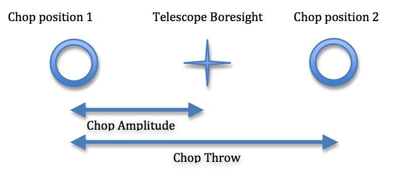
Fig. 67 Symmetric Chop

Asymmetric chopping means that the secondary is aligned with the telescope boresight in one position, but is tilted away from the boresight in the chop position. The chop amplitude is equal to the chop throw in this case (see Fig. 68).

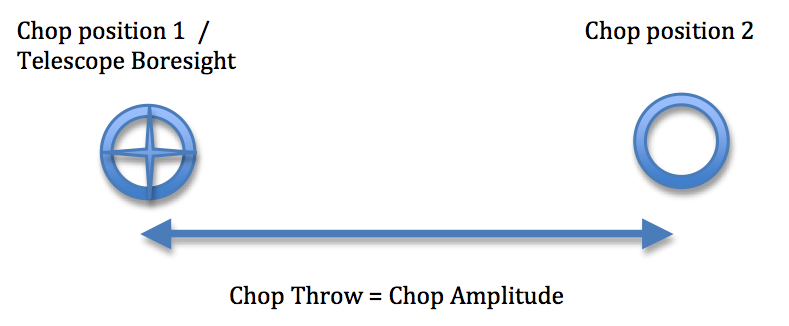
Fig. 68 Asymmetric Chop

Unfortunately, moving the secondary mirror causes the telescope to be slightly misaligned, which introduces optical distortions (notably the optical aberration known as coma) and additional background emission from the telescope (considerably smaller than the sky emission but present nonetheless) in the images. The optical distortions can be minimized by tilting the secondary only tiny fractions of a degree. The additional telescopic background can be removed by moving the entire telescope to a new position and then chopping the secondary again between two positions. Subtracting the two chop images at this new telescope position will remove the sky emission but leave the additional telescopic background due to the misalignment; subtracting the result from the chop-subtracted image at the first telescope position will then remove the background. Since the process of moving to a new position is needed to remove the additional background from the telescope, not the sky, it can be done on a much longer timescale. The variation in the telescopic backgrounds occurs on timescales on the order of tens of seconds to minutes, much slower than the variation in the sky emission.

This movement of the entire telescope, on a much longer timescale than chopping, is known as nodding. The two nod positions are usually referred to as nod A and nod B. The distance between the two nod positions is known as the nod throw or the nod amplitude. For FORCAST observations, nods are done every 5 to 30 seconds. The chop-subtracted images at nod position B are then subtracted from the chop-subtracted images at nod position A. The result will be an image of the region, without the sky background emission or the additional emission resulting from tilting the secondary during the chopping process. The sequence of chopping in one telescope position, nodding, and chopping again in a second position is known as a chop/nod cycle.

Again, because the MIR sky is so bright, deep images of a region cannot be obtained (as they are in the optical) by simply observing the region for a long time with the detector collecting photons continuously. As stated above, the observations require chopping and nodding at fairly frequent intervals. Hence, deep observations are made by “stacking” a series of chop/nod images. Furthermore, MIR detectors are not perfect, and often have bad pixels or flaws. In order to avoid these defects on the arrays, and prevent them from marring the final images, observers employ a technique known as “dithering.” Dithering entails moving the position of the telescope slightly with respect to the center of the region observed each time a new chop/nod cycle is begun, or after several chop/nod cycles. When the images are processed, the observed region will appear in a slightly different place on the detector. This means that the bad pixels do not appear in the same place relative to the observed region. The individual images can then be registered and averaged or median-combined, a process that will eliminate (in theory) the bad pixels from the final image.

Available chopping modes

Symmetric chopping modes: C2N and C2ND

FORCAST acquires astronomical observations in two symmetric chopping modes: two-position chopping with no nodding (C2) and two-position chopping with nodding (C2N). Dithering can be implemented for either mode; two-position chopping with nodding and dithering is referred to as C2ND. The most common observing methods used are C2N and C2ND. C2ND is conceptually very similar to the C2N mode: the only difference is a slight movement of the telescope position after each chop/nod cycle.

FORCAST can make two types of C2N observations: Nod Match Chop (NMC) and Nod Perpendicular to Chop (NPC). The positions of the telescope boresight, the two chop positions, and the two nod positions for these observing types are shown below (Fig. 69 through Fig. 74).

C2N: Nod Match Chop (NMC)

In the NMC mode, the telescope is pointed at a position half of the chop throw distance away from the object to be observed, and the secondary chops between two positions, one of which is centered on the object. The nod throw has the same magnitude as the chop throw, and is in a direction exactly 180 degrees from that of the chop direction. The final image is generated by subtracting the images obtained for the two chop positions at nod A and those at nod B, and then subtracting the results. This will produce three images of the star, one positive and two negative, with the positive being twice as bright as the negatives.

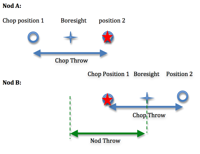
Fig. 69 Nod Match Chop mode

For grism observations, the chop and nod angles can be set relative to the sky or the array (slit). There are two special angles when using the array coordinate system: parallel to (along; Fig. 70), and orthogonal (perpendicular; Fig. 71) to the slit. Dithers should be done along the slit.

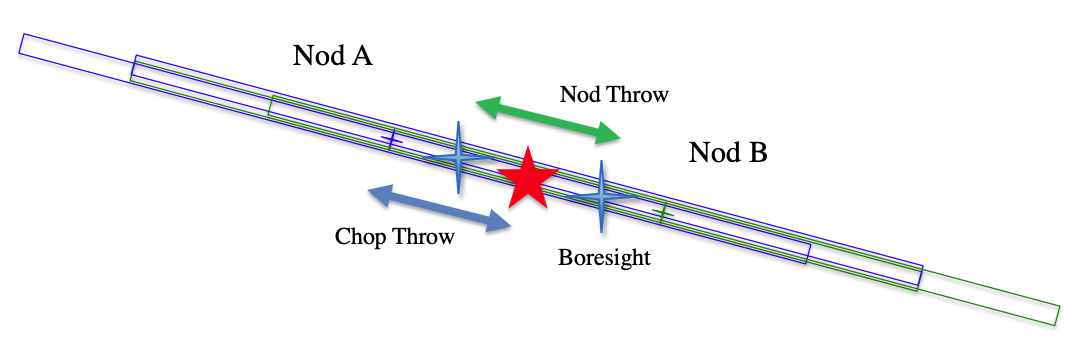
Fig. 70 Nod Match Chop Parallel to Slit

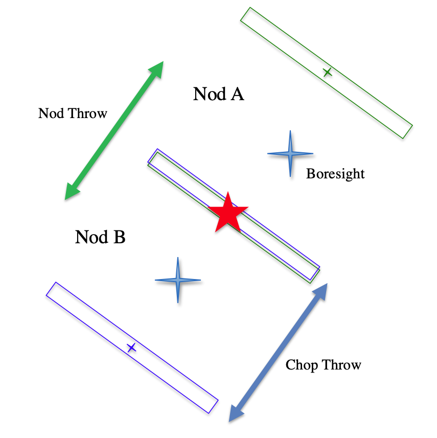
Fig. 71 Nod Match Chop Perpendicular to Slit

C2N: Nod Perpendicular to Chop (NPC)

In the NPC mode, the telescope is offset by half the nod throw from the target in a direction perpendicular to the chop direction, and the secondary chops between two positions. The nod throw usually (but not necessarily) has the same magnitude as the chop, but it is in a direction perpendicular to the chop direction. The final image is generated by subtracting the images obtained for the two chop positions at nod A and those at nod B, and then subtracting the results. This will produce four images of the star in a rectangular pattern, with the image values alternating positive and negative.

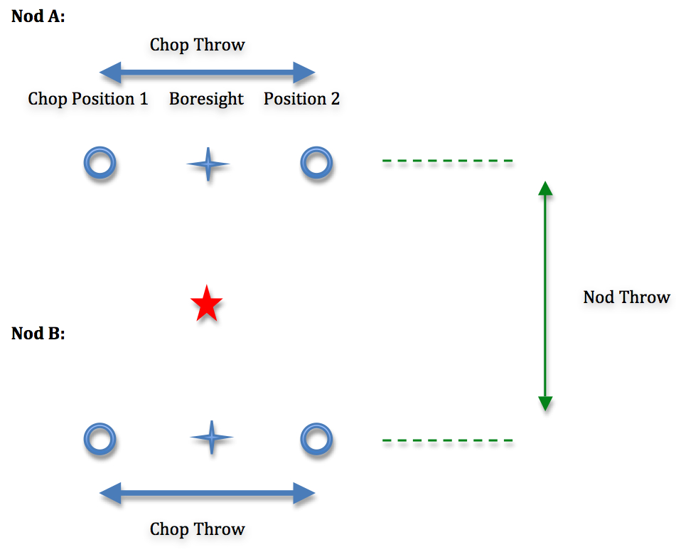
Fig. 72 Nod Perpendicular to Chop mode

For grism observations, there are two types of NPC observations: Chop Along Slit and Nod Along Slit. For Chop Along Slit (Fig. 73), the telescope is pointed at the object and the secondary chops between two positions on either side of the object. The chop throw is oriented such that both positions are aligned with the angle of the slit on the sky. For Nod Along Slit, (Fig. 74) the telescope is pointed at a position half of the chop throw distance away from the object to be observed, and the secondary chops between two positions, one of which is centered on the object. The nod throw is oriented such that both nod positions are aligned with the angle of the slit on the sky.

Fig. 73 Nod Perpendicular to Chop, Chop Along Slit

Fig. 74 Nod Perpendicular to Chop, Nod Along Slit

Asymmetrical chopping modes: C2NC2 and NXCAC

FORCAST also has an asymmetrical chop mode, known as C2NC2. In this mode, the telescope is first pointed at the target (position A). In this first position, the secondary is aligned with the boresight for one observation and then is tilted some amount (often 180-480 arcseconds) for the second (asymmetrically chopped) observation. This is an asymmetric C2 mode observation. The telescope is then slewed some distance from the target, to a sky region without sources (position B), and the asymmetric chop pattern is repeated. The time between slews is typically 30 seconds.

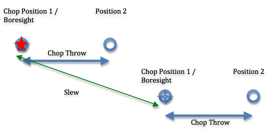
Fig. 75 C2NC2 mode

There is an additional asymmetric mode chopping mode, called NXCAC (nod not related to chop/asymmetrical chop; Fig. 76). This mode replaces the C2NC2 mode when the GI wants to use an asymmetrical chop for a grism observation. This mode is taken with an ABBA nod pattern, like the C2N mode (not ABA, like C2NC2). The nods are packaged together, so data from this mode will reduce just like the C2N mode. The reason for adding this mode stems from the need to define our large chops and nods in ERF (equatorial reference frame), and dither in SIRF (science instrument reference frame) along the slit.

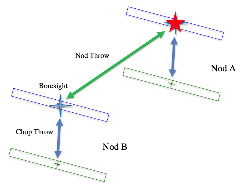
Fig. 76 NXCAC mode

Spectral imaging mode: SLITSCAN

Similar to the C2ND mode for imaging, the SLITSCAN mode for grism observations allows a combination of chopping and nodding with telescope moves to place the spectral extraction slit at different locations in the sky.

In slit-scan observations, a chop/nod cycle is taken at a series of positions, moving the slit slowly across an extended target after each cycle. In this mode, the different telescope positions may be used to generate both extracted spectra at each position and a spatial/spectral cube that combines all the observations together into a spectral map of the source.

Algorithm Description

Overview of data reduction steps

This section will describe, in general terms, the major algorithms that the FORCAST Redux pipeline uses to reduce a FORCAST observation.

The pipeline applies a number of corrections to each input file, regardless of the chop/nod mode used to take the data. The initial steps used for imaging and grism modes are nearly identical; points where the results or the procedure differ for either mode are noted in the descriptions below. After preprocessing, individual images or spectra of a source must be combined to produce the final data product. This procedure depends strongly on the instrument configuration and chop/nod mode.

See Fig. 77 and Fig. 78 for flowcharts of the processing steps used by the imaging and grism pipelines.

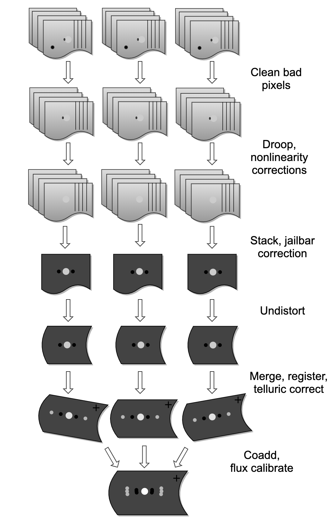
Fig. 77 Processing steps for imaging data.

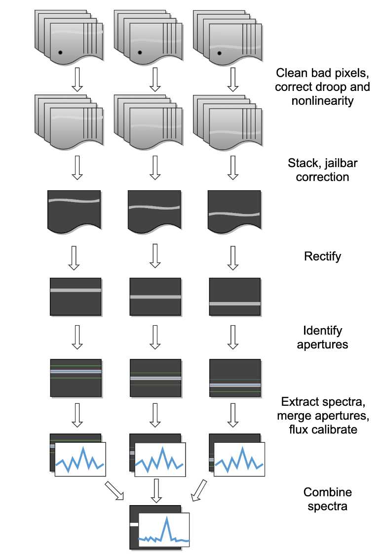
Fig. 78 Processing steps for grism data.

Reduction algorithms

The following subsections detail each of the data reduction pipeline steps:

• Steps common to imaging and spectroscopy modes

  • Identify/clean bad pixels

  • Correct droop effect

  • Correct for detector nonlinearity

  • Subtract background (stack chops/nods)

  • Remove jailbars (correct for crosstalk)

• Imaging-specific steps

  • Correct for optical distortion

  • Merge chopped/nodded images

  • Register images

  • Correct for atmospheric transmission (telluric correct)

  • Coadd multiple observations

  • Calibrate flux

• Spectroscopy-specific steps

  • Stack common dithers

  • Rectify spectral image

  • Identify apertures

  • Extract spectra

  • Merge apertures

  • Calibrate flux and correct for atmospheric transmission

  • Combine multiple observations, or generate response spectra

Steps common to imaging and spectroscopy modes

Identify bad pixels

Bad pixels in the FORCAST arrays take the form of hot pixels (with extreme dark current) or pixels with very different response (usually much lower) than the surrounding pixels. The pipeline minimizes the effects of bad pixels by using a bad pixel mask to identify their locations and then replacing the bad pixels with NaN values. Optionally, the bad pixels may instead be interpolated over, using nearby good values as input.

The bad pixel map for both FORCAST channels is currently produced manually, independent of the pipeline. The mask is a 256x256 image with pixel value = 0 for bad pixels and pixel value = 1 otherwise.

Correct droop effect

The FORCAST arrays and readout electronics exhibit a linear response offset caused by the presence of a signal on the array. This effect is called ‘droop’ since the result is a reduced signal. Droop results in each pixel having a reduced signal that is proportional to the total signal in the 15 other pixels in the row read from the multiplexer simultaneously with that pixel. The effect, illustrated in Fig. 79, is an image with periodic spurious sources spread across the array rows. The droop correction removes the droop offset by multiplying each pixel by a value derived from the sum of every 16th pixel in the same row all multiplied by an empirically determined offset fraction: droopfrac = 0.0035. This value is a configurable parameter, as some data may require a smaller droop fraction to avoid over-correction of the effect. Over-correction may look like an elongated smear along the horizontal axis, near a bright source (see Fig. 80). Note that while droop correction typically removes the effect near the source, there may be lingering artifacts in other areas of the image if the source was very bright, as in Fig. 79.

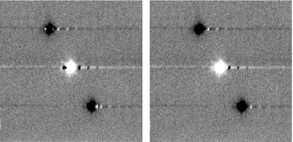
Fig. 79 Background-subtracted FORCAST images of a bright star with droop effect (left) and with the droop correction applied (right).

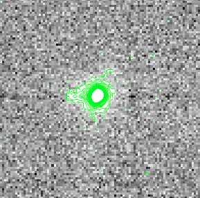
Fig. 80 Overcorrected droop effect, appearing as an elongated smear on the bright central source.

Correct for detector nonlinearity

In principle, the response of each of the pixels in the FORCAST detector arrays should be linear with incident flux. In practice, the degree to which the detector is linear depends on the level of charge in the wells relative to the saturation level. Empirical tests optimizing signal-to-noise indicate that signal levels in the neighborhood of 60% of full well for a given detector capacitance in the FORCAST arrays have minimal departures from linear response and optimal signal-to-noise. For a given background level we can keep signal levels near optimal by adjusting the detector readout frame rate and detector capacitance. Since keeping signals near 60% of saturation level is not always possible or practical, we have measured response curves (response in analog-to-digital units (ADU) as a function of well depth for varying background levels) that yield linearity correction factors. These multiplicative correction factors linearize the response for a much larger range of well depths (about 15% - 90% of saturation). The linearity correction is applied globally to FORCAST images prior to background subtraction. The pipeline first calculates the background level for a sub-image, and then uses this level to calculate the linearity correction factor. The pipeline then applies the correction factor to the entire image.

Subtract background (stack chops/nods)

Background subtraction is accomplished by subtracting chopped image pairs and then subtracting nodded image pairs.

For C2N/NPC imaging mode with chop/nod on-chip (i.e. chop throws smaller than the FORCAST field of view), the four chop/nod images in the raw data file are reduced to a single stacked image frame with a pattern of four background-subtracted images of the source, two positive and two negative. For chop/nod larger than the FORCAST field of view the raw files are reduced to a single frame with one background-subtracted image of the source.

For the C2N/NPC spectroscopic mode, either the chop or the nod is always off the slit, so there will be two traces in the subtracted image: one positive and one negative. If the chop or nod throw is larger than the field of view, there will be a single trace in the image.

In the case of the C2N/NMC mode for either imaging or spectroscopy, the nod direction is the same as the chop direction with the same throw so that the subtracted image frame contains three background-subtracted images of the source. The central image or trace is positive and the two outlying images are negative. If the chop/nod throw is larger than the FORCAST field of view, there will be a single image or trace in the image.

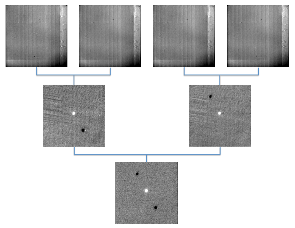
Fig. 81 Images at two stages of background subtraction in imaging NMC mode: raw frames (upper row), chop-subtracted (middle row), chop/nod-subtracted (lower row). Four raw frames produce a single stacked image.

C2NC2 raw data sets for imaging or spectroscopy consist of a set of 5 FITS files, each with 4 image planes containing the chop pairs for both the on-source position (position A) and the blank sky position (position B). The four planes can be reduced in the same manner as any C2N image by first subtracting chopped image pairs for both and then subtracting nodded image pairs. The nod sequence for C2NC2 is \(A_1 B_1 A_2 A_3 B_2 A_4 A_5 B_3\), where the off-source B nods are shared between some of the files (shared B beams shown in bold):

File 1 = \(A_1 \boldsymbol{B_1}\)

File 2 = \(\boldsymbol{B_1} A_2\)

File 3 = \(A_3 \boldsymbol{B_2}\)

File 4 = \(\boldsymbol{B_2} A_4\)

File 5 = \(A_5 \boldsymbol{B_3}\)

The last step in the stack pipeline step is to convert pixel data from analog-to-digital units (ADU) per frame to mega-electrons per second (Me/s) using the gain and frame rate used for the observation.

At this point, the background in the chop/nod-subtracted stack should be zero, but if there is a slight mismatch between the background levels in the individual frames, there may still remain some small residual background level. After stacking, the pipeline estimates this residual background by taking the mode or median of the image data in a central section of the image, and then subtracts this level from the stacked image. This correction is typically not applied for grism data, as the spectroscopic pipeline has other methods for removing residual background.

Remove jailbars (correct for crosstalk)

The FORCAST array readout circuitry has a residual, or latent, signal that persists when pixels have high contrast relative to the surrounding pixels. This can occur for bad pixels or for bright point sources. This residual is present not only in the affected pixels, but is correlated between all pixels read by the same one of sixteen multiplexer channels. This results in a linear pattern of bars, spaced by 16 pixels, known as “jailbars” in the background-subtracted (stacked) images (see Fig. 82). Jailbars can interfere with subsequent efforts to register multiple images since the pattern can dominate the cross-correlation algorithm sometimes used in image registration. The jailbars can also interfere with photometry in images and with spectral flux in spectroscopy frames.

The pipeline attempts to remove jailbar patterns from the background-subtracted images by replacing pixel values by the median value of pixels in that row that are read by the same multiplexer channel (i.e. every 16th pixel in that row starting with the pixel being corrected). The jailbar pattern is located by subtracting a 1-dimensional (along rows) median filtered image from the raw image.

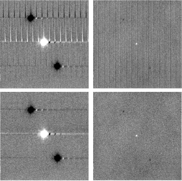
Fig. 82 Crosstalk correction for a bright point source (left), and faint source (right). Images on the top are before correction; images on the bottom are after correction.

Imaging-specific steps

Correct for optical distortion

The FORCAST optical system introduces anamorphic magnification and barrel distortion in the images. The distortion correction uses pixel coordinate offsets for a grid of pinholes imaged in the lab and a 2D polynomial warping function to resample the 256x256 pixels to an undistorted grid. The resulting image is 262x247 pixels with image scale of 0.768”/pixel for a corrected field of view of 3.4x3.2 arcminutes. Pixels outside of the detector area are set to NaN to distinguish them from real data values.

Merge chopped/nodded images

The stack step of the pipeline in imaging mode may produce images with multiple positive and negative source images, depending on the chop/nod mode used for data acquisition. These positive and negative sources may be merged by copying, shifting, and re-combining the image in order to increase the signal-to-noise of the observation. The final image is then rotated by the nominal sky angle, so that North is up and East is left in the final image (see Fig. 83).

The merge pipeline step makes a number of copies of the stacked image, shifts them by the chop and nod throws used in data acquisition, and adds or subtracts them (depending on whether the image is a positive or negative background-subtracted image). The pipeline can use two different methods for registration in the merge process: chop/nod offset data from the FITS header, or centroid of the brightest point source in the stacked images.

The default for flux standards is to use centroiding, as it is usually the most precise method. If merging is desired for science images that do not contain a bright, compact source, the header data method is usually the most reliable. After the shifting and adding, the final merged image consists of a positive image of the source surrounded by a number of positive and negative residual source images left over from the merging process. The central image is the source to use for science.

For the NPC imaging mode with chop/nod amplitude smaller than the field of view, the stack step produces a single stacked image frame with a pattern of four background-subtracted images of the source, two of them negative. The merge step makes four copies of the stacked frame, then shifts each using the selected algorithm. It adds or subtracts each copy, depending on whether the source is positive or negative.

For the NMC imaging mode with chop/nod amplitude smaller than the field of view, the stacked image contains three background-subtracted sources, two negative, and one positive (see Fig. 81). The positive source has double the flux of the negative ones, since the source falls in the same place on the detector for two of the chop/nod positions. The merge step for this mode makes three copies of the image, shifts the two negative sources on top of the positive one, and then subtracts them (see Fig. 83). Pixels with no data are set to NaN.

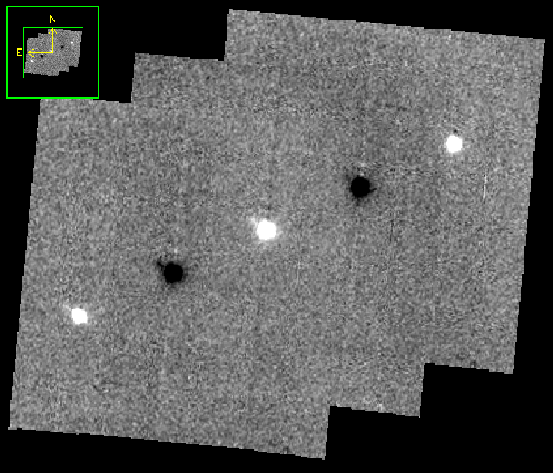
Fig. 83 The NMC observation of Fig. 81, after merging. Only the central source should be used for science; the other images are artifacts of the stacking and merging procedure. Note that the merged image is rotated to place North up and East left.

While performing the merge, the locations of overlap for the shifted images are recorded. For NPC mode, the final merged image is normalized by dividing by the number of overlapping images at each pixel. For NMC mode, because the source is doubled in the stacking step, the final merged image is divided by the number of overlapping images, plus one. In the nominal case, if all positive and negative sources were found and coadded, the signal in the central source, in either mode, should now be the average of four observations of the source. If the chop or nod was relatively wide, however, and one or more of the extra sources were not found on the array, then the central source may be an average of fewer observations.

For either NPC or NMC imaging modes, with chop/nod amplitude greater than half of the array, there is no merging to be done, as the extra sources are off the detector. However, for NMC mode, the data is still divided by 2 to account for the doubled central source. For C2NC2 mode, the chops and telescope moves-to-sky are always larger than the FORCAST field of view; merging is never required for this mode. It may also be desirable to skip the merging stage for crowded fields-of-view and extended sources, as the merge artifacts may be confused with real sources.

In all imaging cases, whether or not the shifting-and-adding is performed, the merged image is rotated by the sky angle at the end of the merge step.

Register images

In order to combine multiple imaging observations of the same source, each image must be registered to a reference image, so that the pixels from each image correspond to the same location on the sky.

The registration information is typically encoded in the world coordinate system (WCS) embedded in each FITS file header. For most observations, the WCS is sufficiently accurate that no change is required in the registration step. However, if the WCS is faulty, it may be corrected in the registration step, using centroiding or cross-correlation between images to identify common sources, or using header information about the dither offsets used. In this case,the first image is taken as the reference image, and calculated offsets are applied to the WCS header keywords (CRPIX1 and CRPIX2) in all subsequent images. [1]

[1]

Earlier versions of this pipeline applied registration to the images themselves, rather than to the WCS in the FITS header, interpolating them into the same spatial grid. As of v2.0.0, registration affects only the CRPIX1 and CRPIX2 keywords in the header.

Correct for atmospheric transmission

For accurate flux calibration, the pipeline must first correct for the atmospheric opacity at the time of the observation. In order to combine images taken in different atmospheric conditions, or at different altitudes or zenith angles, the pipeline corrects the flux in each individual registered file for the estimated atmospheric transmission during the observations, based on the altitude and zenith angle at the time when the observations were obtained, relative to that computed for a reference altitude (41,000 feet) and reference zenith angle (45 degrees), for which the instrumental response has been calculated. The atmospheric transmission values are derived from the ATRAN code provided to the SOFIA program by Steve Lord. The pipeline applies the telluric correction factor directly to the flux in the image, and records it in the header keyword TELCORR.

After telluric correction, the pipeline performs aperture photometry on all observations that are marked as flux standards (FITS keyword OBSTYPE = STANDARD_FLUX). The brightest source in the field is fit with a Moffat profile to determine its centroid, and then its flux is measured, using an aperture of 12 pixels and a background region of 15-25 pixels. The aperture flux and error, as well as the fit characteristics, are recorded in the FITS header, to be used in the flux calibration process.

Coadd multiple observations

After registration and scaling, the pipeline coadds multiple observations of the same source with the same instrument configuration and observation mode. Each image is projected into the coordinate system of the first image, using its WCS to transform input coordinates into output coordinates. An additional offset may be applied for non-sidereal targets in order to correct for the motion of the target across the sky, provided that the target position is recorded in the FITS headers (TGTRA and TGTDEC). The projection is performed with a bilinear interpolation, then individual images are mean- or median-combined, with optional error weighting and robust outlier rejection.

For flux standards, photometry calculations are repeated on the coadded image, in the same way they were performed on the individual images.

Calibrate flux

For the imaging mode, flux calibration factors are typically calculated from all standards observed within a flight series. These calibration factors are applied directly to the flux images to produce an image calibrated to physical units. The final Level 3 product has image units of Jy per pixel. [2]

See the flux calibration section, below, for more information.

[2]

Earlier versions of this pipeline did not produce a final calibrated file. Prior to v1.1.0, the final Level 3 products had image units of Me/sec, with the flux calibration factor (Me/sec/Jy) recorded in the FITS header keyword, CALFCTR. To convert these products to Jy/pixel, divide the flux image by the CALFCTR value.

Mosaic

In some cases, it may be useful to stack together separate calibrated observations of the same target. In order to create a deeper image of a faint target, for example, observations taken across multiple flights may be combined together. Large maps may also be generated by taking separate observations, and stitching together the results. In these cases, the pipeline may register these files and coadd them, using the same methods as in the initial registration and coadd steps. The output product is a LEVEL_4 mosaic.

Spectroscopy-specific steps

Stack common dithers

For very faint spectra, a second stacking step may be optionally performed. This step identifies spectra at common dither positions and mean- or median-combines them in order to increase signal-to-noise. This step may be applied if spectra are too faint to automatically identify appropriate apertures.

Rectify spectral image

For the spectroscopic mode, spatial and spectral distortions are corrected for by defining calibration images that assign a wavelength coordinate (in \(\mu m\)) and a spatial coordinate (in arcsec) to each detector pixel, for each grism available. Each 2D spectral image in an observation is resampled into a rectified spatial-spectral grid, using these coordinates to define the output grid. If appropriate calibration data is available, the output from this step is an image in which wavelength values are constant along the columns, and spatial values are constant along the rows, correcting for any curvature in the spectral trace (Fig. 84).

These calibration maps are generated from identifications of sky emission and telluric absorption lines and a polynomial fit to centroids of those features in pixel space for each row (i.e. along the dispersion direction). The derivation of a wavelength calibration is an interactive process, but application of the derived wavelength calibration is an automatic part of the data reduction pipeline. The default wavelength calibration is expected to be good to within approximately one pixel in the output spectrum.

For some observational cycles, sufficient calibration data may not be available, resulting in some residual spectral curvature, or minor wavelength calibration inaccuracies. The spectral curvature can be compensated for, in sources with strong continuum emission, by tracing the continuum center during spectral extraction (see next section). For other sources, a wider aperture may be set, at the cost of decreased signal-to-noise.

For NMC observations, the central spectrum is doubled in flux after stacking, as for imaging NMC modes. After the rectified image is generated, it is divided by 2 for NMC mode data, in order to normalize the flux value. [3]

Additionally, a correction that accounts for spatial variations in the instrumental throughput may be applied to the rectified image. This “slit correction function” is a function of the position of the science target spectrum along the slit relative to that used for the standard stars. The slit function image is produced in a separate calibration process, from observations of sources taken at varying places on the slit.

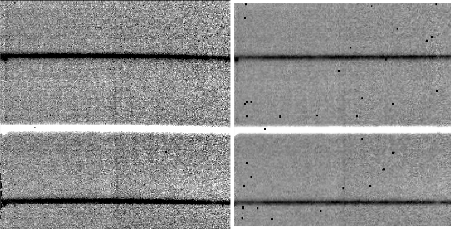
Fig. 84 A NMC spectral image, before (left) and after (right) rectification. The black spots indicate bad pixels, identified with NaN values. Bad pixel influence grows during the resampling process in rectification.

[3]

Earlier versions of this pipeline deferred this normalization to later steps. In pipeline versions prior to v1.4.0, the ‘rectimg’ product (*RIM*.fits) was not normalized for NMC data: it should be divided by 2 before being used for spectral extractions.

Identify apertures

In order to aid in spectral extraction, the pipeline constructs a smoothed model of the relative intensity of the target spectrum at each spatial position, for each wavelength. This spatial profile is used to compute the weights in optimal extraction or to fix bad pixels in standard extraction (see next section). Also, the pipeline uses the median profile, collapsed along the wavelength axis, to define the extraction parameters.

To construct the spatial profile, the pipeline first subtracts the median signal from each column in the rectified spectral image to remove the residual background. The intensity in this image in column i and row j is given by

\(O_{ij} = f_{i}P_{ij}\)

where \(f_i\) is the total intensity of the spectrum at wavelength i, and \(P_{ij}\) is the spatial profile at column i and row j. To get the spatial profile \(P_{ij}\), we must approximate the intensity \(f_i\). To do so, the pipeline computes a median over the wavelength dimension (columns) of the order image to get a first-order approximation of the median spatial profile at each row \(P_j\). Assuming that

\(O_{ij} \approx c_{i}P_{j}\),

the pipeline uses a linear least-squares algorithm to fit \(P_j\) to \(O_{ij}\) and thereby determine the coefficients \(c_i\). These coefficients are then used as the first-order approximation to \(f_i\): the resampled order image \(O_{ij}\) is divided by \(f_i\) to derive \(P_{ij}\). The pipeline then fits a low-order polynomial along the columns at each spatial point s in order to smooth the profile and thereby increase its signal-to-noise. The coefficients of these fits can then be used to determine the value of \(P_{ij}\) at any column i and spatial point j (see Fig. 85, left). The median of \(P_{ij}\) along the wavelength axis generates the median spatial profile, \(P_j\) (see Fig. 85, right).

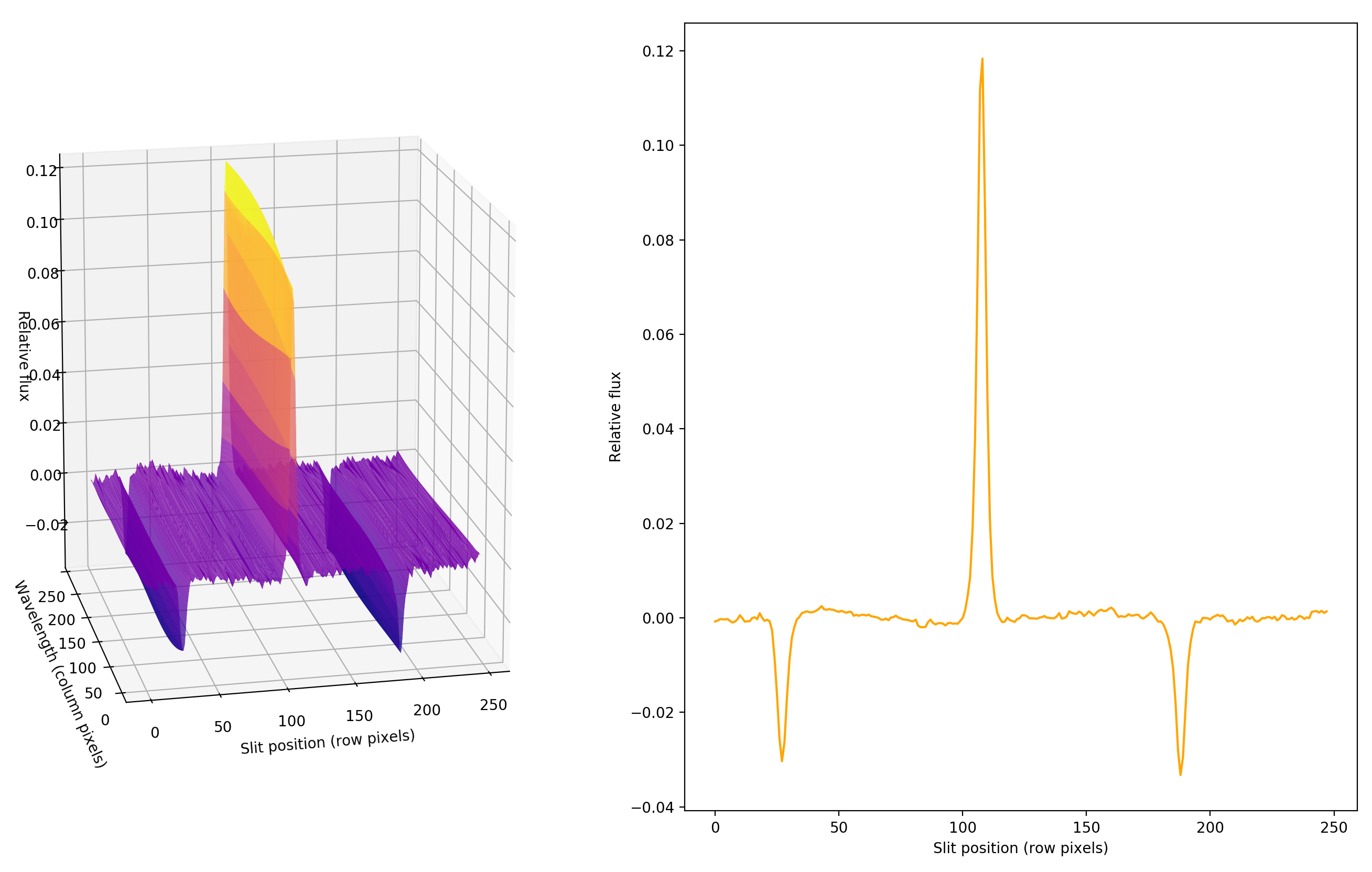
Fig. 85 Spatial model and median spatial profile, for the image in Fig. 84. The spatial model image here is rotated for comparison with the profile plot: the y-axis is along the bottom of the surface plot; the x-axis is along the left.

The pipeline then uses the median spatial profile to identify extraction apertures for the source. The aperture centers can be identified automatically by iteratively finding local maxima in the absolute value of the spatial profile, or can be specified directly by the user. By default, a single aperture is expected and defined by the pipeline, but additional apertures may also be defined (e.g. for NMC or NPC spectra with chopping or nodding on-slit, as in Fig. 84).

The true position of the aperture center may vary somewhat with wavelength, as a result of small optical effects or atmospheric dispersion. To account for this variation, the pipeline attempts to trace the spectrum across the array. It fits a Gaussian in the spatial direction, centered at the specified position, at regular intervals in wavelength. The centers of these fits are themselves fitted with a low-order polynomial; the coefficients of these fits give the trace coefficients that identify the center of the spectral aperture at each wavelength. For extended sources, the continuum cannot generally be directly traced. Instead, the pipeline fixes the aperture center to a single spatial value.

Besides the aperture centers, the pipeline also specifies a PSF radius, corresponding to the distance from the center at which the flux from the source falls to zero. This value is automatically determined from the width of a Gaussian fit to the peak in the median spatial profile, as

\(R_{psf} = 2.15 \cdot \text{FWHM}\).

For optimal extraction, the pipeline also identifies a smaller aperture radius, to be used as the integration region:

\(R_{ap} = 0.7 \cdot \text{FWHM}\).

This value should give close to optimal signal-to-noise for a Moffat or Gaussian profile. The pipeline also attempts to specify background regions outside of any extraction apertures, for fitting and removing the residual sky signal. All aperture parameters may be optionally overridden by the pipeline user.

Spectral extraction and merging

The spectral extraction algorithms used by the pipeline offer two different extraction methods, depending on the nature of the target source. For point sources, the pipeline uses an optimal extraction algorithm, described at length in the Spextool paper (see the Other Resources section, below, for a reference). For extended sources, the pipeline uses a standard summing extraction.

In either method, before extracting a spectrum, the pipeline first uses any identified background regions to find the residual sky background level. For each column in the 2D image, it fits a low-order polynomial to the values in the specified regions, as a function of slit position. This polynomial determines the wavelength-dependent sky level (\(B_{ij}\)) to be subtracted from the spectrum (\(D_{ij}\)).

The standard extraction method uses values from the spatial profile image (\(P_{ij}\)) to replace bad pixels and outliers, then sums the flux from all pixels contained within the PSF radius. The flux at column i is then:

\(f_{i,\text{sum}} = \sum_{j=j_1}^{j_2}(D_{ij} - B_{ij})\)

where \(j_1\) and \(j_2\) are the upper and lower limits of the extraction aperture (in pixels):

\(j_1 = t_i - R_{PSF}\)

\(j_2 = t_i + R_{PSF}\)

given the aperture trace center (\(t_i\)) at that column. This extraction method is the only algorithm available for extended sources.

Point sources may occasionally benefit from using standard extraction, but optimal extraction generally produces higher signal-to-noise ratios for these targets. This method works by weighting each pixel in the extraction aperture by how much of the target’s flux it contains. The pipeline first normalizes the spatial profile by the sum of the spatial profile within the PSF radius defined by the user:

\(P_{ij}^{'} = P_{ij} \Big/ \sum_{j=j_1}^{j_2}P_{ij}\).

\(P_{ij}^{'}\) now represents the fraction of the total flux from the target that is contained within pixel (i,j), so that \((D_{ij} - B_{ij}) / P_{ij}^{'}\) is a set of j independent estimates of the total flux at column i. The pipeline does a weighted average of these estimates, where the weight depends on the pixel’s variance and the normalized profile value. Then, the flux at column i is:

\(f_{i,\text{opt}} = \frac{\sum_{j=j_3}^{j_4}{M_{ij}P_{ij}^{'}(D_{ij} - B_{ij}) \big/ (V_{D_{ij}} + V_{B_{ij}})}}{\sum_{j=j_3}^{j_4}{M_{ij}{P_{ij}^{'}}^{2} \big/ (V_{D_{ij}} + V_{B_{ij}})}}\)

where \(M_{ij}\) is a bad pixel mask and \(j_3\) and \(j_4\) are the upper and lower limits given by the aperture radius:

\(j_3 = t_i - R_{ap}\)

\(j_4 = t_i + R_{ap}\)

Note that bad pixels are simply ignored, and outliers will have little effect on the average because of the weighting scheme.

After extraction, spectra from separate apertures (e.g. for NMC mode, with chopping on-slit) may be merged together to increase the signal-to-noise of the final product. The default combination statistic is a robust weighted mean.

Calibrate flux and correct for atmospheric transmission

Extracted spectra are corrected individually for instrumental response and atmospheric transmission, a process that yields a flux-calibrated spectrum in units of Jy per pixel. See the section on flux calibration, below, for more detailed information.

The rectified spectral images are also corrected for atmospheric transmission, and calibrated to physical units in the same manner. Each row of the image is divided by the same correction as the 1D extracted spectrum. This image is suitable for custom extractions of extended fields: a sum over any number of rows in the image produces a flux-calibrated spectrum of that region, in the same units as the spectrum produced directly by the pipeline.

Note that the FITS header for the primary extension for this product (PRODTYPE = ‘calibrated_spectrum’) [4] contains a full spatial and spectral WCS that can be used to identify the coordinates of any spectra so extracted. The primary WCS identifies the spatial direction as arcseconds up the slit, but a secondary WCS with key = ‘A’ identifies the RA, Dec, and wavelength of every pixel in the image. Either can be extracted and used for pixel identification with standard WCS manipulation packages, such as the astropy WCS package.

[4]

In early versions of the pipeline (before v1.4.0), the calibrated rectified image was not produced. For versions 1.4.0 to 1.5.0, the product type was PRODTYPE = ‘calrectimg’, and it contained only the calibrated image. For version 2.0.0 and higher, the product type is ‘calibrated_spectrum’, and the calibrated image and associated WCS are contained in the primary extension. Subsequent extensions also contain the calibrated extracted spectra and reference atmospheric transmission and response spectra.

After telluric correction, it is possible to apply a correction to the calibrated wavelengths for the motion of the Earth relative to the solar system barycenter at the time of the observation. For FORCAST resolutions, we expect this wavelength shift to be a small fraction of a pixel, well within the wavelength calibration error, so we do not directly apply it to the data. The shift (as \(d\lambda / \lambda\)) is calculated and stored in the header in the BARYSHFT keyword. An additional wavelength correction to the local standard of rest (LSR) from the barycentric velocity is also stored in the header, in the LSRSHFT keyword.

Combine multiple observations

The final pipeline step for most grism observation modes is coaddition of multiple spectra of the same source with the same instrument configuration and observation mode. The individual extracted 1D spectra are combined with a robust weighted mean, by default. The 2D spectral images are also coadded, using the same algorithm as for imaging coaddition, and the spatial/spectral WCS to project the data into a common coordinate system.

Reductions of flux standards have an alternate final product (see Response spectra, below). Slit-scan observations also produce an alternate final product instead of directly coadding spectra (see Spectral cubes, below).

Response spectra

The final product of pipeline processing of telluric standards is not a calibrated, combined spectrum, but rather an instrumental response spectrum that may be used to calibrate science target spectra. These response spectra are generated from individual observations of calibration sources by dividing the observed spectra by a model of the source multiplied by an atmospheric model. The resulting response curves may then be combined with other response spectra from a flight series to generate a master instrument response spectrum that is used in calibrating science spectra. See the flux calibration section, below, for more information.

Spectral cubes

For slit-scan observations, the calibrated, rectified images produced at the flux calibration step are resampled together into a spatial/spectral cube.

Since the pipeline rectifies all images onto the same wavelength grid, each column in the image corresponds to the same wavelength in all rectified images from the same grism. The pipeline uses the WCS in the headers to assign a spatial position to each pixel in each input image, then steps through the wavelength values, resampling the spatial values into a common grid.

The resampling algorithm proceeds as follows. At each wavelength value, the algorithm loops over the output spatial grid, finding values within a local fitting window. Values within the window are fit with a low-order polynomial surface fit. These fits are weighted by the error on the flux, as propagated by the pipeline, and by a Gaussian function of the distance from the data point to the grid location. The output flux at each pixel is the value of the surface polynomial, evaluated at the grid location. The associated error value is the error on the fit. Grid locations for which there was insufficient input data are set to NaN. An exposure map cube indicating the number of observations input at each pixel is also generated and attached to the output FITS file.

Uncertainties

The pipeline calculates the expected uncertainties for raw FORCAST data as an error image associated with the flux data. FORCAST raw data is recorded in units of ADU per coadded frame. The variance associated with the (i,j)th pixel in this raw data is calculated as:

\[V_{ij} = \frac{N_{ij} \beta_g}{\text{FR} \cdot t \cdot g} + \frac{\text{RN}^2}{\text{FR} \cdot t \cdot g^2}\]

where \(N\) is the raw ADU per frame in each pixel, \(\beta_g\) is the excess noise factor, \(FR\) is the frame rate, \(t\) is the integration time, \(g\) is the gain, and \(RN\) is the read noise in electrons. The first term corresponds to the Poisson noise, and the second to the read noise. Since FORCAST data are expected to be background-limited, the Poisson noise term should dominate the read noise term. The error image is the square root of \(V_{ij}\) for all pixels.

For all image processing steps and spectroscopy steps involving spectral images, the pipeline propagates this calculated error image alongside the flux in the standard manner. The error image is written to disk as an extra extension in all FITS files produced at intermediate steps. [5]

The variance for the standard spectroscopic extraction is a simple sum of the variances in each pixel within the aperture. For the optimal extraction algorithm, the variance on the ith pixel in the extracted spectrum is calculated as:

\[V_{i} = \sum_{j=j_3}^{j_4} \frac{M_{ij}}{{P_{ij}^{'}}^2 V_{ij}}\]

where \(P_{ij}^{'}\) is the scaled spatial profile, \(M_{ij}\) is a bad pixel mask, \(V_{ij}\) is the variance at each background-subtracted pixel, and the sum is over all spatial pixels \(j\) within the aperture radius. This equation comes from the Spextool paper, describing optimal extraction. The error spectrum for 1D spectra is the square root of the variance.

[5]

In pipeline versions prior to v2.0.0, the error was stored as a variance image, as a second plane in the primary FITS image extension. In versions 2.0.0 and later, each FITS image extension has a distinct scientific meaning: flux and error images are stored as 2D data arrays, in separate extensions. Refer to the BUNIT keyword for the physical units of the data stored in each extension.

Other Resources

For more information about the pipeline software architecture and implementation, see the FORCAST Redux Developer’s Manual.

For more information on the spectroscopic reduction algorithms used in the pipeline, see the Spextool papers:

Spextool: A Spectral Extraction Package for SpeX, a 0.8-5.5 micron Cross-Dispersed Spectrograph

Michael C. Cushing, William D. Vacca and John T. Rayner (2004, PASP 116, 362).

A Method of Correcting Near-Infrared Spectra for Telluric Absorption

William D. Vacca, Michael C. Cushing and John T. Rayner (2003, PASP 115, 389).

Nonlinearity Corrections and Statistical Uncertainties Associated with Near-Infrared Arrays

William D. Vacca, Michael C. Cushing and John T. Rayner (2004, PASP 116, 352).

Flux calibration

Imaging Flux Calibration

The reduction process, up through image coaddition, generates Level 2 images with data values in units of mega-electrons per second (Me/s). After Level 2 imaging products are generated, the pipeline derives the flux calibration factors (in units of Me/s/Jy) and applies them to each image. The calibration factors are derived for each FORCAST filter configuration (filter and dichroic) from observations of calibrator stars.

After the calibration factors have been derived, the coadded flux is divided by the appropriate factor to produce the Level 3 calibrated data file, with flux in units of Jy/pixel. The value used is stored in the FITS keyword CALFCTR.

Reduction steps

The calibration is carried out in several steps. The first step consists of measuring the photometry of all the standard stars for a specific mission or flight series, after the images have been corrected for the atmospheric transmission relative to that for a reference altitude and zenith angle [6]. The pipeline performs aperture photometry on the reduced Level 2 images of the standard stars after the registration stage using a photometric aperture radius of 12 pixels (about 9.2” for FORCAST). The telluric-corrected photometry of the standard star is related to the measured photometry of the star via

\[N_{e}^{std,corr} = N_{e}^{std} \frac{R_{\lambda}^{ref}}{R_{\lambda}^{std}}\]

where the ratio \(R_{\lambda}^{ref} / R_{\lambda}^{std}\) accounts for differences in system response (atmospheric transmission) between the actual observations and those for the reference altitude of 41000 feet and a telescope elevation of 45\(^\circ\). Similarly, for the science target, we have

\[N_{e}^{obj,corr} = N_{e}^{obj} \frac{R_{\lambda}^{ref}}{R_{\lambda}^{obj}}\]

Calibration factors (in Me/s/Jy) for each filter are then derived from the measured photometry (in Me/s) and the known fluxes of the standards (in Jy) in each filter. These predicted fluxes were computed by multiplying a model stellar spectrum by the overall filter + instrument + telescope + atmosphere (at the reference altitude and zenith angle) response curve and integrating over the filter passband to compute the mean flux in the band. The adopted filter throughput curves are those provided by the vendor or measured by the FORCAST team, modified to remove regions (around 6-7 microns and 15 microns) where the values were contaminated by noise. The instrument throughput is calculated by multiplying the transmission curves of the entrance window, dichroic, internal blockers, and mirrors, and the detector quantum efficiency. The telescope throughput value is assumed to be constant (85%) across the entire FORCAST wavelength range.

For most of the standard stars, the adopted stellar models were obtained from the Herschel calibration group and consist of high-resolution theoretical spectra, generated from the MARCS models (Gustafsson et al. 1975, Plez et al. 1992), scaled to match absolutely calibrated observational fluxes (Dehaes et al. 2011). For \(\beta\) UMi, the model was scaled by a factor of 1.18 in agreement with the results of the Herschel calibration group (J. Blommaert, private communication; the newer version of the model from the Herschel group has incorporated this factor).

The calibration factor, C, is computed from

\[C = \frac{N_e^{std,corr}}{F_{\nu}^{nom,std}(\lambda_{ref})} = \frac{N_e^{std,corr}}{\langle F_{\nu}^{std} \rangle} \frac{\lambda^2_{piv}}{\langle \lambda \rangle \lambda_{ref}}\]

with an uncertainty given by

\[\bigg( \frac{\sigma_C}{C} \bigg)^2 = \bigg( \frac{\sigma_{N_e^{std}}}{N_e^{std}} \bigg)^2 + \bigg( \frac{\sigma_{\langle F_{\nu}^{std} \rangle}}{\langle F_{\nu}^{std} \rangle} \bigg)^2 .\]

Here, \(\lambda_{piv}\) is the pivot wavelength of the filter, and \(\langle \lambda \rangle\) is the mean wavelength of the filter. The calibration factor refers to a nominal flat spectrum source at the reference wavelength \(\lambda_{ref}\).

The calibration factors derived from each standard for each filter are then averaged. The pipeline inserts this value and its associated uncertainty into the headers of the Level 2 data files for the flux standards, and uses the value to produce calibrated flux standards. The final step involves examining the calibration values and ensuring that the values are consistent. Outlier values may come from bad observations of a standard star; these values are removed to produce a robust average of the calibration factor across the flight series. The resulting average values are then used to calibrate the observations of the science targets.

Using the telluric-corrected photometry of the standard, \(N_e^{std,corr}\) (in Me/s), and the predicted mean fluxes of the standards in each filter, \(\langle F_{\nu}^{std} \rangle\) (in Jy), the flux of a target object is given by

\[F_{\nu}^{nom,obj}(\lambda_{ref}) = \frac{N_e^{obj,corr}}{C}\]

where \(N_e^{obj,corr}\) is the telluric-corrected count rate in Me/s detected from the source, \(C\) is the calibration factor (Me/s/Jy), and \(F_{\nu}^{nom,obj}(\lambda_{ref})\) is the flux in Jy of a nominal, flat spectrum source (for which \(F_{\nu} \sim \nu^{-1}\)) at a reference wavelength \(\lambda_{ref}\).

The values of \(C\), \(\sigma_C\), and \(\lambda_{ref}\) are written into the headers of the calibrated (PROCSTAT=LEVEL_3 ) data as the keywords CALFCTR, ERRCALF, and LAMREF, respectively. The reference wavelength \(\lambda_{ref}\) for these observations was taken to be the mean wavelengths of the filters, \(\langle \lambda \rangle\).

Note that \(\sigma_C\), as stored in the ERRCALF value, is derived from the standard deviation of the calibration factors across multiple flights. These values are typically on the order of about 6% (see Herter et al. 2013). There is an additional systematic uncertainty on the stellar models, which is on the order of 5-10% (Dehaes et al. 2011).

[6]

The atmospheric transmission in each filter has been computed using the ATRAN code (Lord 1992) for a range of observatory altitudes (corresponding to a range of overhead precipitable water vapor values) and telescope elevations. The ratio of the transmission at each altitude and zenith angle relative to that at the reference altitude (41000 feet) and zenith angle (45 degrees) has been calculated for each filter and fit with a low order polynomial. The ratio appropriate for the altitude and zenith angle of each observation is calculated and applied to each image.

Color corrections

An observer often wishes to determine the true flux of an object at the reference wavelength, \(F_{\nu}^{obj}(\lambda_{ref})\), rather than the flux of an equivalent nominal, flat spectrum source. To do this, we define a color correction K such that

\[K = \frac{F_{\nu}^{nom,obj}(\lambda_{ref})}{F_{\nu}^{obj}(\lambda_{ref})}\]

where \(F_{\nu}^{nom,obj}(\lambda_{ref})\) is the flux density obtained by measurement on a data product. Divide the measured values by K to obtain the “true” flux density. In terms of the wavelengths defined above,

\[K = \frac{\langle \lambda \rangle \lambda_{ref}}{\lambda_{piv}^2}\frac{\langle F_{\nu}^{obj} \rangle}{F_{\nu}^{obj}(\lambda_{ref})} .\]

For most filters and spectral shapes, the color corrections are small (<10%). Tables listing K values and filter wavelengths are available from the SOFIA website.

Spectrophotometric Flux Calibration

The common approach to characterizing atmospheric transmission for ground-based infrared spectroscopy is to obtain, for every science target, similar observations of a spectroscopic standard source with as close a match as possible in both airmass and time. Such an approach is not practical for airborne observations, as it imposes too heavy a burden on flight planning and lowers the efficiency of science observations. Therefore, we employ a calibration plan that incorporates a few observations of a calibration star per flight and a model of the atmospheric absorption for the approximate altitude and airmass (and precipitable water vapor, if known) at which the science objects were observed.

Instrumental response curves are generated from the extracted spectra of calibrator targets. For the G063 and G111 grisms, the calibrator targets comprise the set of standard stars and the associated stellar models provided by the Herschel Calibration program and used for the FORCAST photometric calibration. For the G227 and G329 grisms, the calibrator targets consist of bright asteroids. Blackbodies are fit to the calibrated broadband photometric observations of the asteroids and these serve as models of the intrinsic asteroid spectra. In either case, the extracted spectra are corrected for telluric absorption using the ATRAN models corresponding to the altitude and zenith angle of the calibrator observations, smoothed to the nominal resolution for the grism/slit combination, and sampled at the observed spectral binning. The telluric-corrected spectra are then divided by the appropriate models to generate response curves (with units of Me/s/Jy at each wavelength) for the various grism+slit+channel combinations. The response curves derived from the various calibrators for each instrumental combination are then combined and smoothed to generate a set of master instrumental response curves. The statistical uncertainties on these response curves are on the order of 5-10%.

Spectra of science targets are first divided by the appropriate instrumental response curve, a process that yields spectra in physical units of Jy at each wavelength.

Telluric correction of FORCAST grism data for a science target is currently carried out in a multi-step process:

1. Telluric absorption models have been computed, using ATRAN, for the entire set of FORCAST grism passbands for every 1000 feet of altitude between 35K and 45K feet, for every 5 degrees of zenith angle between 30 and 70 degrees, and for a set of precipitable water vapor (PWV) values between 1 and 50 microns. These values span the allowed ranges of zenith angle, typical range of observing altitudes, and the expected range of PWV values for SOFIA observations. The spectra have been smoothed to the nominal resolution for the grism and slit combination and are resampled to the observed spectral binning.

2. If the spectrum of the science target has a signal-to-noise ratio greater than 10, the best estimate of the telluric absorption spectrum is derived in the following manner: under the assumption that the intrinsic low-resolution MIR spectrum of most targets can be well-represented by a smooth, low-order polynomial, the telluric spectrum that minimizes \(\chi^2\) defined as

   \[\chi_j^2 = \sum\limits_i^n \Big( F_i^{obs} - P_i T_i \big(\text{PWV}_j \big) \Big)^2 \big/ \sigma_i^2\]

   is determined. Here \(F_i^{obs}\) is the response-corrected spectrum at each of the n wavelength points i, \(\sigma_i\) is the uncertainty at each point, \(P_i\) is the polynomial at each point, and \(T_i\) is the telluric spectrum corresponding to the precipitable water vapor value \(\text{PWV}_j\). The telluric spectra used in the calculations are chosen from the pre-computed library generated with ATRAN. Only the subset of ATRAN model spectra corresponding, as close as possible, to the observing altitude and zenith angle, are considered in the calculation. The free parameters determined in this step are the coefficients of the polynomial and the PWV value, which then yields the best telluric correction spectrum. The uncertainty on the PWV value is estimated to be about 1-2 microns.

3. If the spectrum of the science target has a S/N less than 10, the closest telluric spectrum (in terms of altitude and airmass of the target observations) with the default PWV value from the ATRAN model is selected from the pre-computed library.

4. In order to account for any wavelength shifts between the models and the observations, an optimal shift is estimated by minimizing the residuals of the corrected spectrum, with respect to small relative wavelength shifts between the observed data and the telluric spectrum.

5. The wavelength-shifted observed spectrum is then divided by the smoothed and re-sampled telluric model. This then yields a telluric-corrected and flux calibrated spectrum.

Analysis of the calibrated spectra of observed standard stars indicates that the average RMS deviation over the G063, G227, and G329 grism passbands between the calibrated spectra and the models is on the order of about 5%. For the G111 grism, the average RMS deviation is found to be on the order of about 10%; the larger deviation for this grism is due primarily to the highly variable ozone feature at 9.6 microns, which the ATRAN models are not able to reproduce accurately. The Level 3 data product for any grism includes the calibrated spectrum and an error spectrum that incorporates these RMS values. The adopted telluric absorption model and the instrumental response functions are also provided.

As for any slit spectrograph, highly accurate absolute flux levels from FORCAST grism observations (for absolute spectrophotometry, for example) require additional photometric observations to correct the calibrated spectra for slit losses that can be variable (due to varying image quality) between the spectroscopic observations of the science target and the calibration standard.

Data products

Filenames

Output files from Redux are named according to the convention:

FILENAME = F[flight]_FO_IMA|GRI_AOR-ID_SPECTEL1|SPECTEL2_Type_FN1[-FN2].fits,

where flight is the SOFIA flight number, FO is the instrument identifier, IMA or GRI specifies that it is an imaging or grism file, AOR-ID is the AOR identifier for the observation, SPECTEL1|SPECTEL2 is the keyword specifying the filter or grism used, Type is three letters identifying the product type (listed in Table 15 and Table 16, below), FN1 is the file number corresponding to the input file. FN1-FN2 is used if there are multiple input files for a single output file, where FN1 is the file number of the first input file and FN2 is the file number of the last input file.

Pipeline Products

The following tables list all intermediate products generated by the pipeline for imaging and grism modes, in the order in which they are produced. [7] By default, for imaging, the undistorted, merged, telluric_corrected, coadded, calibrated, and mosaic products are saved; for grism, the stacked, rectified_image, merged_spectrum, calibrated_spectrum, coadded_spectrum, and combined_spectrum products are saved.

The final grism mode output product from the Combine Spectra or Combine Response steps are dependent on the input data: for INSTMODE=SLITSCAN, a spectral_cube product is produced instead of a coadded_spectrum and combined_spectrum; for OBSTYPE=STANDARD_TELLURIC, the instrument_response is produced instead.

For most observation modes, the pipeline additionally produces an image in PNG format, intended to provide a quick-look preview of the data contained in the final product. These auxiliary products may be distributed to observers separately from the FITS file products.

[7]

Earlier versions of this pipeline (before v2.0.0) produced different sets of default products. Refer to earlier revisions of this manual for complete information.

Table 15 Intermediate data products for imaging reductions

Step	Data type	PRODTYPE	PROCSTAT	Code	Saved	Extensions
Clean Images	2D image	cleaned	LEVEL_2	CLN	N	FLUX, ERROR
Correct Droop	2D image	drooped	LEVEL_2	DRP	N	FLUX, ERROR
Correct Nonlinearity	2D image	linearized	LEVEL_2	LNZ	N	FLUX, ERROR
Stack Chops/Nods	2D image	stacked	LEVEL_2	STK	N	FLUX, ERROR
Undistort	2D image	undistorted	LEVEL_2	UND	Y	FLUX, ERROR
Merge	2D image	merged	LEVEL_2	MRG	Y	FLUX, ERROR, EXPOSURE
Register	2D image	registered	LEVEL_2	REG	N	FLUX, ERROR, EXPOSURE
Telluric Correct	2D image	telluric_ corrected	LEVEL_2	TEL	Y	FLUX, ERROR, EXPOSURE
Coadd	2D image	coadded	LEVEL_2	COA	Y	FLUX, ERROR, EXPOSURE
Flux Calibrate	2D image	calibrated	LEVEL_3	CAL	Y	FLUX, ERROR, EXPOSURE
Mosaic	2D image	mosaic	LEVEL_4	MOS	Y	FLUX, ERROR, EXPOSURE

Table 16 Intermediate data products for spectroscopy reduction

Step	Data type	PRODTYPE	PROCSTAT	Code	Saved	Extensions
Clean Images	2D spectral image	cleaned	LEVEL_2	CLN	N	FLUX, ERROR
Correct Droop	2D spectral image	drooped	LEVEL_2	DRP	N	FLUX, ERROR
Correct Nonlinearity	2D spectral image	linearized	LEVEL_2	LNZ	N	FLUX, ERROR
Stack Chops/Nods	2D spectral image	stacked	LEVEL_2	STK	Y	FLUX, ERROR
Make Profiles	2D spectral image	rectified_ image	LEVEL_2	RIM	Y	FLUX, ERROR, BADMASK, WAVEPOS, SLITPOS, SPATIAL_MAP, SPATIAL_PROFILE
Locate Apertures	2D spectral image	apertures_ located	LEVEL_2	LOC	N	FLUX, ERROR, BADMASK, WAVEPOS, SLITPOS, SPATIAL_MAP, SPATIAL_PROFILE
Trace Continuum	2D spectral image	continuum_ traced	LEVEL_2	TRC	N	FLUX, ERROR, BADMASK, WAVEPOS, SLITPOS, SPATIAL_MAP, SPATIAL_PROFILE, APERTURE_TRACE
Set Apertures	2D spectral image	apertures_set	LEVEL_2	APS	N	FLUX, ERROR, BADMASK, WAVEPOS, SLITPOS, SPATIAL_MAP, SPATIAL_PROFILE, APERTURE_TRACE, APERTURE_MASK
Subtract Background	2D spectral image	background_ subtracted	LEVEL_2	BGS	N	FLUX, ERROR, BADMASK, WAVEPOS, SLITPOS, SPATIAL_MAP, SPATIAL_PROFILE, APERTURE_TRACE, APERTURE_MASK
Extract Spectra	2D spectral image; 1D spectrum	spectra	LEVEL_2	SPM	N	FLUX, ERROR, BADMASK, WAVEPOS, SLITPOS, SPATIAL_MAP, SPATIAL_PROFILE, APERTURE_TRACE, APERTURE_MASK, SPECTRAL_FLUX, SPECTRAL_ERROR, TRANSMISSION
Merge Apertures	2D spectral image; 1D spectrum	merged_ spectrum	LEVEL_2	MGM	Y	FLUX, ERROR, BADMASK, WAVEPOS, SLITPOS, SPATIAL_MAP, SPATIAL_PROFILE, APERTURE_TRACE, APERTURE_MASK, SPECTRAL_FLUX, SPECTRAL_ERROR, TRANSMISSION
Calibrate Flux	2D spectral image; 1D spectrum	calibrated_ spectrum	LEVEL_3	CRM	Y	FLUX, ERROR, BADMASK, WAVEPOS, SLITPOS, SPATIAL_MAP, SPATIAL_PROFILE, APERTURE_TRACE, APERTURE_MASK, SPECTRAL_FLUX, SPECTRAL_ERROR TRANSMISSION, RESPONSE, RESPONSE_ERROR
Combine Spectra	2D spectral image; 1D spectrum	coadded_ spectrum	LEVEL_3	COA	Y	FLUX, ERROR, EXPOSURE, WAVEPOS, SPECTRAL_FLUX, SPECTRAL_ERROR TRANSMISSION, RESPONSE
Combine Spectra	1D spectrum	combined_ spectrum	LEVEL_3	CMB	Y	FLUX
Combine Spectra	3D spectral cube	spectral_ cube	LEVEL_4	SCB	Y	FLUX, ERROR, EXPOSURE, WAVEPOS, TRANSMISSION, RESPONSE
Make Response	1D response spectrum	response_ spectrum	LEVEL_3	RSP	Y	FLUX
Combine Response	1D response spectrum	instrument_ response	LEVEL_4	IRS	Y	FLUX

Data Format

All files produced by the pipeline are multi-extension FITS files (except for the combined_spectrum, response_spectrum, and instrument_response products: see below). [8] The flux image is stored in the primary header-data unit (HDU); its associated error image is stored in extension 1, with EXTNAME=ERROR. For the spectral_cube product, these extensions contain 3D spatial/spectral cubes instead of 2D images: each plane in the cube represents the spatial information at a wavelength slice.

Imaging products may additionally contain an extension with EXTNAME=EXPOSURE, which contains the nominal exposure time at each pixel, in seconds. This extension has the same meaning for the spectroscopic coadded_spectrum and spectral_cube products.

In spectroscopic products, the SLITPOS and WAVEPOS extensions give the spatial (rows) and spectral (columns) coordinates, respectively, for rectified images. These coordinates may also be derived from the WCS in the primary header. WAVEPOS also indicates the wavelength coordinates for 1D extracted spectra.

Intermediate spectral products may contain SPATIAL_MAP and SPATIAL_PROFILE extensions. These contain the spatial map and median spatial profile, described in the Rectify spectral image section, above. They may also contain APERTURE_TRACE and APERTURE_MASK extensions. These contain the spectral aperture definitions, as described in the Identify apertures section.

Final spectral products contain SPECTRAL_FLUX and SPECTRAL_ERROR extensions: these are the extracted 1D spectrum and associated uncertainty. They also contain TRANSMISSION and RESPONSE extensions, containing the atmospheric transmission and instrumental response spectra used to calibrate the spectrum (see the Calibrate flux and correct for atmospheric transmission section).

The combined_spectrum, response_spectrum, and instrument_response are one-dimensional spectra, stored in Spextool format, as rows of data in the primary extension.

For the combined_spectrum, the first row is the wavelength (um), the second is the flux (Jy), the third is the error (Jy), the fourth is the estimated fractional atmospheric transmission spectrum, and the fifth is the instrumental response curve used in flux calibration (Me/s/Jy). These rows correspond directly to the WAVEPOS, SPECTRAL_FLUX, SPECTRAL_ERROR, TRANSMISSION, and RESPONSE extensions in the coadded_spectrum product.

For the response_spectrum, generated from telluric standard observations, the first row is the wavelength (um), the second is the response spectrum (Me/s/Jy), the third is the error on the response (Me/s/Jy), the fourth is the atmospheric transmission spectrum (unitless), and the fifth is the standard model used to derive the response (Jy). The instrument_reponse spectrum, generated from combined response_spectrum files, similarly has wavelength (um), response (Me/s/Jy), error (Me/s/Jy), and transmission (unitless) rows.

The final uncertainties in calibrated images and spectra contain only the estimated statistical uncertainties due to the noise in the image or the extracted spectrum. The systematic uncertainties due to the calibration process are recorded in header keywords. For imaging data, the error on the calibration factor is recorded in the keyword ERRCALF. For grism data, the estimated overall fractional error on the flux is recorded in the keyword CALERR. [9]

[8]

In earlier versions of this pipeline (prior to 2.0.0), all image products were 3D arrays of data, where the first plane was the image and the second plane was the variance associated with each pixel in the image. The square root of the variance plane gives the uncertainty estimate associated with each pixel in the image. An optional third plane was the exposure map, indicating the on-source integration time in seconds at each pixel. All spectral products were in the Spextool format described above for the combined_spectrum product.

[9]

Earlier versions of this pipeline (prior to 1.2.0) may have stored the systematic calibration error in the error spectrum or variance image, added in quadrature with the statistical error. Check PIPEVERS and compare the error estimates for the calibrated products to earlier products to ensure correct interpretation of the error estimates.

Data Quality

Data quality for FORCAST is recorded in the FITS keyword DATAQUAL and can contain the following values:

• NOMINAL: No outstanding issues with processing, calibration, or observing conditions.

• USABLE: Minor issue(s) with processing, calibration, or conditions but should still be scientifically valid (perhaps with larger than usual uncertainties); see HISTORY records for details.

• PROBLEM: Significant issue(s) encountered with processing, calibration, or observing conditions; may not be scientifically useful (depending on the application); see HISTORY records for details. In general, these cases are addressed through manual reprocessing before archiving and distribution.

• FAIL: Data could not be processed successfully for some reason. These cases are rare and generally not archived or distributed to the GI.

Any issues found in the data or during flight are recorded as QA Comments and emailed to the GI after processing and archiving. A permanent record of these comments are also directly recorded in the FITS files themselves. Check the FITS headers, near the bottom of the HISTORY section, under such titles as “Notes from quality analysis” or “QA COMMENTS”.

Other data quality keywords include CALQUAL and WCSQUAL. The CALQUAL keyword may have the following values:

• NOMINAL: Calibration is within nominal historical variability of 5-10%.

• USABLE: Issue(s) with calibration. Variability is greater than nominal limits, but still within the maximum requirements (<20%).

• PROBLEM: Significant issue(s) with calibration variability (>20%), or inability to properly calibrate. Data may not be scientifically useful.

The keyword WCSQUAL refers to the quality of the World Coordinate System (WCS) for astrometry. In very early FORCAST cycles, there were many issues with astrometry, as described in the Known Issues document. Astrometry could, in the worst cases, be off by a full chop- or nod-throw distance (up to hundreds of pixels/arcseconds). These issues were resolved in Cycle 3 and 4. However, there still appears to be a slight distortion of 1-2 pixels across the FORCAST Field of View (FOV) (where one FORCAST pixel is 0.768 arcsec). Methodologies to reduce this distortion are currently being worked on. In addition, cooling of the telescope mirror system exposed to the Stratosphere over the course of a night observing can also result in a pointing accuracy change on order of 1-2 pixels. Thus, is it important in cases where very accurate astrometry is required that FORCAST data be checked relative to other observations. This can also affect large mosaics of regions of the sky where, depending on the changing rotation angle on sky, overlapping sources may be slightly misaligned due to the distortion across the FOV. Due to these issues the majority of data is set to a WCSQUAL value of UNKNOWN. Values for the WCSQUAL keyword are described below:

• NOMINAL: No issues with chop/nod position miscalculation; WCS matches requested coordinates to within accuracy limits.

• PROBLEM: The WCS reference position deviates from the requested coordinates by more than 1 pixel.

• UNKNOWN: WCS has not been confirmed, however beginning in Cycle 4, are expected to match requested coordinates to within accuracy limits.

Exposure Time

FORCAST has many keywords for time of integration with slightly different interpretation, including EXPTIME, TOTINT, and DETITIME. Due to the details of the setup for chop/nod observations in symmetric and asymmetric modes, the various integration times may not appear to match what was calculated using SOFIA Instrument Time Estimator (SITE). From Cycle 10 onwards, SITE will be updated so that all times use EXPTIME and the mode (C2NC2, NMC, etc.) will be selectable for a better estimate of the observing time required. See below for a comparison of the total time keywords by observing mode.

Table 17 Integration time keywords

Mode	EXPTIME	TOTINT
NMC (shift and add negative beams, e.g. standards)	2 × DETITIME	2 × DETITIME
NMC (no shift and add, only use positive beam)	1 × DETITIME	2 × DETITIME
C2NC2/NXCAC	0.5 × DETITIME	0.5 × DETITIME

Pipeline Updates

The FORCAST data reduction pipeline software has gone through several updates over time and is constantly improving. In particular, the recent update to version 2.0.0 introduced some relatively large changes to the format of the data that may require updates to any local routines used to analyze the data.

Below is a table summarizing major changes by pipeline version. Dates refer to approximate release dates. Check the PIPEVERS key in FITS headers to confirm the version used to process the data, as some early data may have been reprocessed with later pipeline versions. More detailed change notes are available in Appendix D: Change notes for the FORCAST pipeline.

Table 18 Pipeline change notes

PIPEVERS	DATE	Software/Cycle	Comments
<1.0.3	01/23/15	IDL:Cycle 1,2	Earliest FORCAST data where some modes were still being commissioned.
1.0.5	05/27/15	IDL:Cycle 3	TOTINT keyword added for comparison to requested/planned value in SITE.
1.1.3	09/20/16	IDL:Cycle 4/5	Update rotation of field to filter boresight rather than center of array; previous data may have had an offset in astrometry between different filters.
1.2.0	01/25/17	IDL:Cycle 4/5	Overall improvement to calibration. Updated to include TEL files which are similar to REG files with telluric corrections applied to each file. Final calibrated file CAL file is same as COA file but with calibration factor (CALFCTR) already applied. Improved telluric correction for FORCAST grism data.
1.3.0	04/24/17	IDL:Cycle 5	Pipeline begins support for FORCAST LEVEL 4 Imaging Mosaics. EXPOSURE map is now propagated in units of time (seconds) instead of number of exposures.
2.0.0	5/07/20	Python:Cycle 8/9	File format of FITS files for imaging updated from image cube to separate extensions. Extensions are now FLUX, ERROR, and EXPOSURE. ERROR now represents the standard deviation (sigma) rather than the variance (sigma^2). Spectroscopy data formats also move to separate extensions, with some products combining spectra and 2D spectral images.

Grouping LEVEL_1 data for processing

In order for a group of imaging data to be reduced together usefully, all images must have the same target object and be taken in the same chop/nod mode. They must also have the same detector, filter, and dichroic setting. In order to be combined together, they must also be taken on the same mission. Optionally, it may also be useful to separate out data files taken from different observation plans.

For spectroscopy, all the same rules hold, with the replacement of grism element for filter, and with the additional requirement that the same slit be used for all data files.

These requirements translate into a set of FITS header keywords that must match in order for a set of data to be grouped together. These keyword requirements are summarized in the tables below.

Table 19 Grouping Criteria: Imaging

Keyword	Data Type	Match Criterion
OBSTYPE	STR	Exact
OBJECT	STR	Exact
INSTCFG	STR	Exact
DETCHAN	STR	Exact
SPECTEL1 / SPECTEL2*	STR	Exact
BORESITE	STR	Exact
DICHROIC	STR	Exact
MISSN-ID (optional)	STR	Exact
PLANID (optional)	STR	Exact
AOR_ID (optional)	STR	Exact

Table 20 Grouping Criteria: Spectroscopy

Keyword	Data Type	Match Criterion
OBSTYPE	STR	Exact
OBJECT	STR	Exact
INSTCFG	STR	Exact
DETCHAN	STR	Exact
SPECTEL1 / SPECTEL2*	STR	Exact
BORESITE	STR	Exact
DICHROIC	STR	Exact
SLIT**	STR	Exact
MISSN-ID (optional)	STR	Exact
PLANID (optional)	STR	Exact
AOR_ID (optional)	STR	Exact

* SPECTEL1 is used if the detector is the SWC (DETCHAN=SW); SPECTEL2 is used for LWC (DETCHAN=LW)

** If SLIT is in use (value != “NONE” or “UNKNOWN”), always include group in the grism plan, regardless of INSTCFG. This ensures that slit images get reduced with the spectroscopic data and placed in the same preview.

Configuration and execution

Installation

The FORCAST pipeline is written entirely in Python. The pipeline is platform independent and has been tested on Linux, Mac OS X, and Windows operating systems. Running the pipeline requires a minimum of 16GB RAM, or equivalent-sized swap file.

The pipeline is comprised of five modules within the sofia_redux package: sofia_redux.instruments.forcast, sofia_redux.pipeline, sofia_redux.calibration, sofia_redux.spectroscopy, sofia_redux.toolkit. The forcast module provides the data processing algorithms specific to FORCAST, with supporting libraries from the toolkit, calibration, and spectroscopy modules. The pipeline module provides interactive and batch interfaces to the pipeline algorithms.

External Requirements

To run the pipeline for any mode, Python 3.8 or higher is required, as well as the following packages: numpy, scipy, matplotlib, pandas, astropy, configobj, numba, bottleneck, joblib, and photutils. Some display functions for the graphical user interface (GUI) additionally require the PyQt5, pyds9, and regions packages. All required external packages are available to install via the pip or conda package managers. See the Anaconda environment file (environment.yml), or the pip requirements file (requirements.txt) distributed with sofia_redux for up-to-date version requirements.

Running the pipeline interactively also requires an installation of SAO DS9 for FITS image display. See http://ds9.si.edu/ for download and installation instructions. The ds9 executable must be available in the PATH environment variable for the pyds9 interface to be able to find and control it. Please note that pyds9 is not available on the Windows platform

Source Code Installation

The source code for the FORCAST pipeline maintained by the SOFIA Data Processing Systems (DPS) team can be obtained directly from the DPS, or from the external GitHub repository. This repository contains all needed configuration files, auxiliary files, and Python code to run the pipeline on FORCAST data in any observation mode.

After obtaining the source code, install the package with the command:

python setup.py install

from the top-level directory.

Alternately, a development installation may be performed from inside the directory with the command:

pip install -e .

After installation, the top-level pipeline interface commands should be available in the PATH. Typing:

redux

from the command line should launch the GUI interface, and:

redux_pipe -h

should display a brief help message for the command line interface.

Configuration

For FORCAST algorithms, default parameter values are defined by the Redux object that interfaces to them. These values may be overridden manually for each step, while running in interactive mode. They may also be overridden by an input parameter file, in INI format, in either interactive or automatic mode. See Appendix A for an example of an input parameter file, which contains the current defaults for all parameters.

Input data

Redux takes as input raw FORCAST FITS data files, which contain image cubes composed of 256x256 pixel image arrays. The number of frames per raw data cube depends on the chop/nod mode used to acquire the data (see Table 21). The FITS headers contain data acquisition and observation parameters and, combined with the pipeline configuration files, comprise the information necessary to complete all steps of the data reduction process. Some critical keywords are required to be present in the raw FITS headers in order to perform a successful grouping, reduction, and ingestion into the SOFIA archive. See Appendix B for a description of these keywords.

Table 21 Contents of FORCAST raw data files by observing mode

Chop/Nod Mode	Number of frames	Comments
C2N, NMC	4	Two-Position Chop with Nod Matched in throw and parallel to the chop direction 2 chop positions in each of 2 nod positions
C2N, NPC	4	Two-Position Chop with Nod perpendicular to the chop direction 2 chop positions in each of 2 nod positions
C2NC2	4	Extreme asymmetric chop and telescope move to blank sky: two chop positions per sky position. Typically 5 input files corresponding to ABAABAAB pattern
N	2	Two-position Nod only, may be used for grism spectroscopy
SLITSCAN	4	Spectral map of an extended source, most likely using C2NC2 but could use C2N

It is assumed that the input data have been successfully grouped before beginning reduction: Redux considers all input files in a reduction to be science files that are part of a single homogeneous reduction group, to be reduced together with the same parameters. As such, when the pipeline reads a raw FORCAST data file, it uses the first input file to identify the observing mode used. Given this information, it identifies a set of auxiliary and calibration data files to be used in the reduction (Table 22). The default files to be used are defined in a lookup table that reads the DATE-OBS keyword from the raw file, and then chooses the appropriate calibrations for that date.

Table 22 Auxiliary files

Auxiliary data file	Data type	Comments
Configuration file (e.g. OC3_dripconf.txt)	ASCII	Contains initial configuration of pipeline parameters and nonlinearity coefficients
Keyword definition file (e.g. OC3_keywords.txt)	ASCII	Contains the definition of required keywords, with allowed value ranges
Bad pixel mask (e.g. swc_badpix.fits)	FITS	Single 2D image containing locations of bad pixels in short wave or long wave camera
Pinhole location table (e.g. pinhole_locs.txt)	ASCII	Pinhole locations file for distortion correction (imaging only)
Reference flux calibration table (e.g. refcalfac_20191025.txt)	ASCII	Flux calibration factor (imaging only)
Spectral order definition file (e.g. G063_LS24_flat.fits)	FITS	Image file containing header keywords that define the edges of all orders in a 2D spectral image (grism only)
Wavelength calibration map (e.g. G063_wavecal_OC3.fits)	FITS	Two frame image associating a wavelength value and a spatial distance across the slit with each pixel (grism only)
Atmospheric transmission curve (e.g. atran_41K_45deg_4-50mum.fits)	FITS	A FITS image with wavelength and transmission values for a particular altitude and zenith angle (grism only)
Instrumental response curve (e.g. G063_LS24_DB175_response.fits)	FITS	FITS image containing the response at each wavelength for a particular grism/slit mode (grism only)
Slit function image (e.g. G063_LS24_slitfn_OC2.fits)	FITS	FITS image containing the slit response, in rectified spectral coordinates (grism only)

Automatic Mode Execution

The DPS pipeline infrastructure runs a pipeline on previously-defined reduction groups as a fully-automatic black box. To do so, it creates an input manifest (infiles.txt) that contains relative paths to the input files (one per line). The command-line interface to the pipeline is run as:

redux_pipe infiles.txt

The command-line interface will read in the specified input files, use their headers to determine the observation mode, and accordingly the steps to run and any intermediate files to save. Output files are written to the current directory, from which the pipeline was called. After reduction is complete, the script will generate an output manifest (outfiles.txt) containing the relative paths to all output FITS files generated by the pipeline.

Optionally, in place of a manifest file, file paths to input files may be directly specified on the command line. Input files may be raw FITS files, or may be intermediate products previously produced by the pipeline. For example, this command will complete the reduction for a set of FITS files in the current directory, previously reduced through the calibration step of the pipeline:

redux_pipe *CAL*.fits

To customize batch reductions from the command line, the redux_pipe interface accepts a configuration file on the command line. This file may contain any subset of the full configuration file, specifying any non-default parameters for pipeline steps. An output directory for pipeline products and the terminal log level may also be set on the command line.

The full set of optional command-line parameters accepted by the redux_pipe interface are:

-h, --help            show this help message and exit
-c CONFIG, --configuration CONFIG
                      Path to Redux configuration file.
-o OUTDIR, --out OUTDIR
                      Path to output directory.
-l LOGLEVEL, --loglevel LOGLEVEL
                      Log level.

Manual Mode Execution

In manual mode, the pipeline may be run interactively, via a graphical user interface (GUI) provided by the Redux package. The GUI is launched by the command:

redux

entered at the terminal prompt (Fig. 86). The GUI allows output directory specification, but it may write initial or temporary files to the current directory, so it is recommended to start the interface from a location to which the user has write privileges.

From the command line, the redux interface accepts an optional config file (-c) or log level specification (-l), in the same way the redux_pipe command does. Any pipeline parameters provided to the interface in a configuration file will be used to set default values; they will still be editable from the GUI.

Fig. 86 Redux GUI startup.

Basic Workflow

To start an interactive reduction, select a set of input files, using the File menu (File->Open New Reduction). This will bring up a file dialog window (see Fig. 87). All files selected will be reduced together as a single reduction set.

Redux will decide the appropriate reduction steps from the input files, and load them into the GUI, as in Fig. 88.

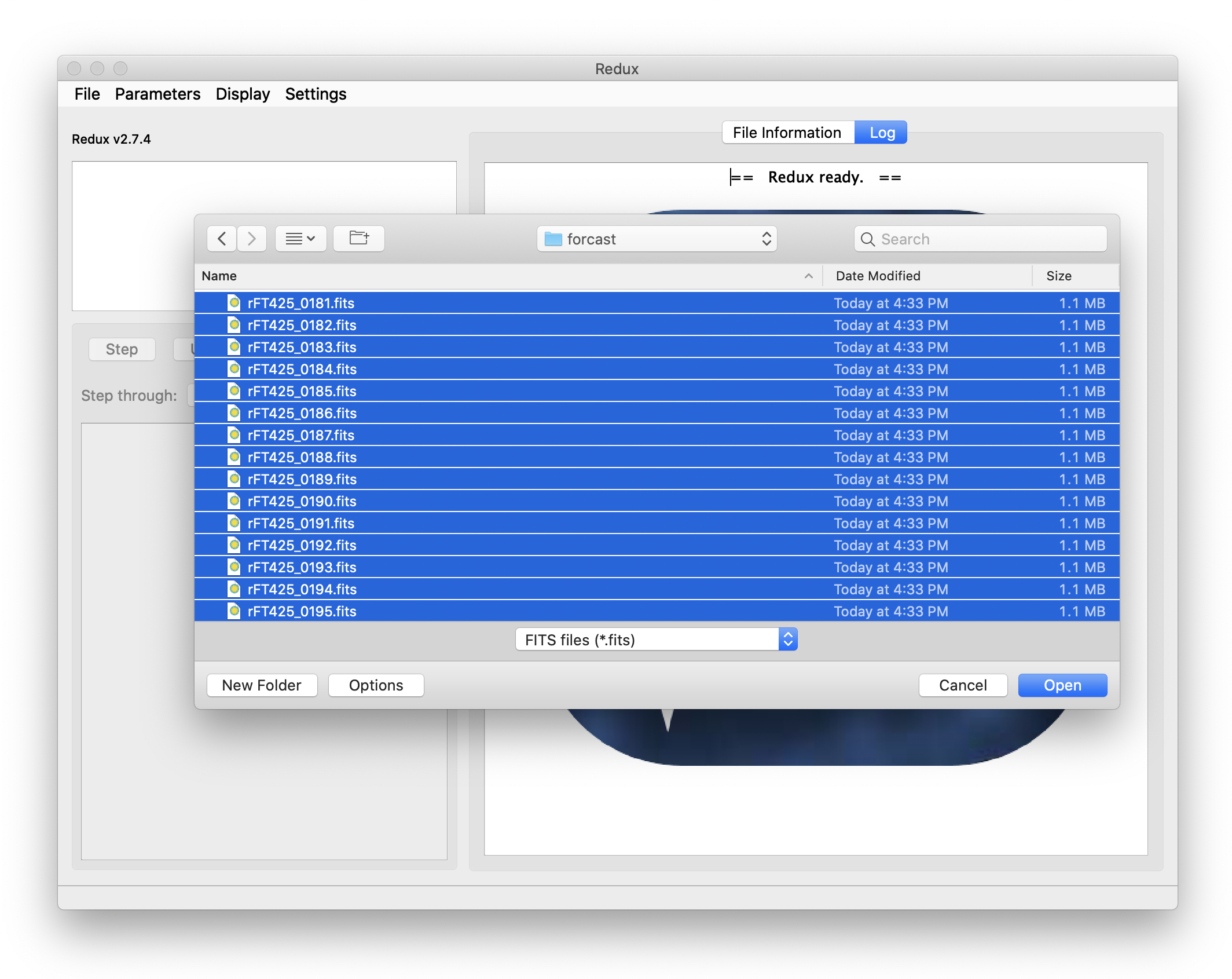
Fig. 87 Open new reduction.

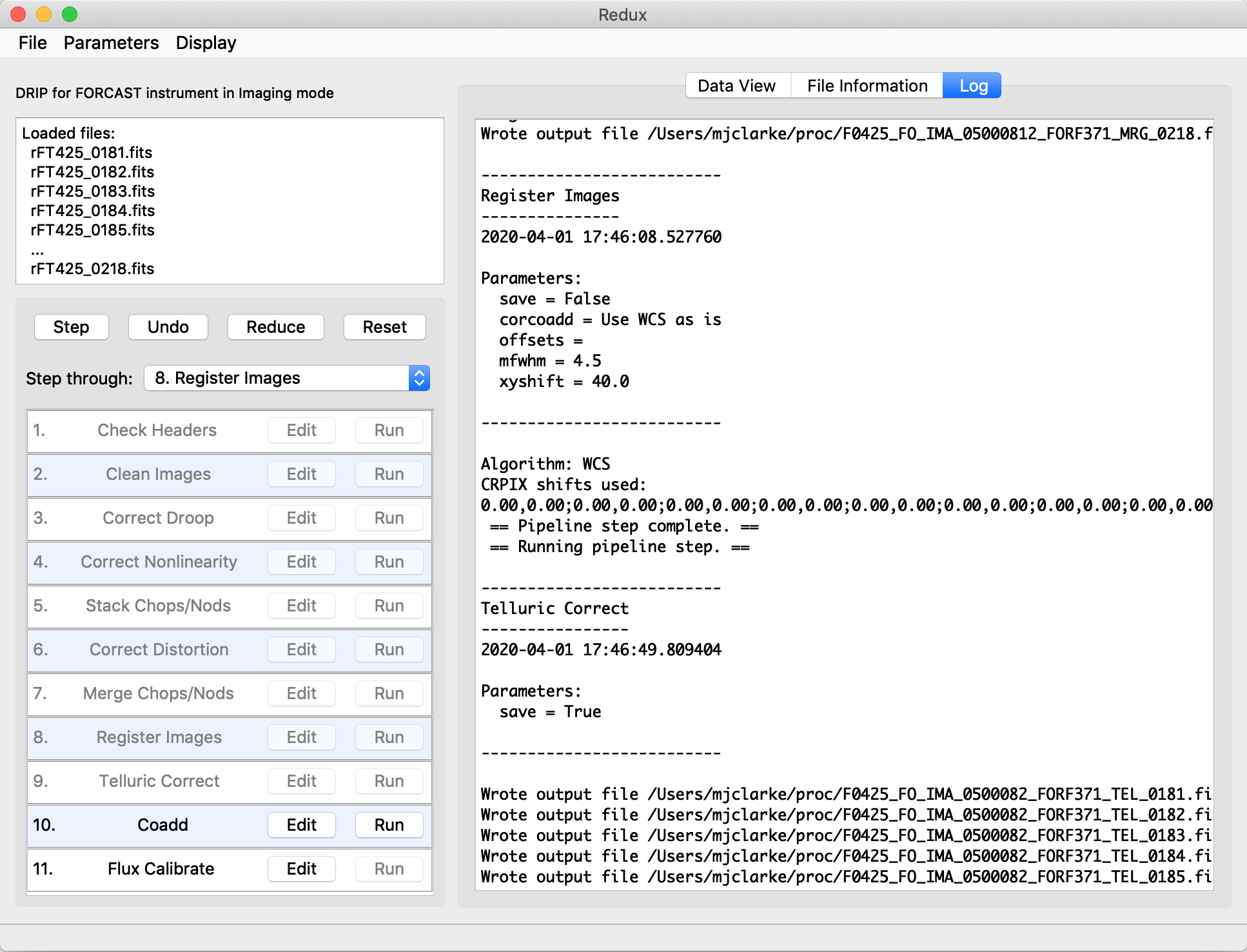
Fig. 88 Sample reduction steps. Log output from the pipeline is displayed in the Log tab.

Each reduction step has a number of parameters that can be edited before running the step. To examine or edit these parameters, click the Edit button next to the step name to bring up the parameter editor for that step (Fig. 89). Within the parameter editor, all values may be edited. Click OK to save the edited values and close the window. Click Reset to restore any edited values to their last saved values. Click Restore Defaults to reset all values to their stored defaults. Click Cancel to discard all changes to the parameters and close the editor window.

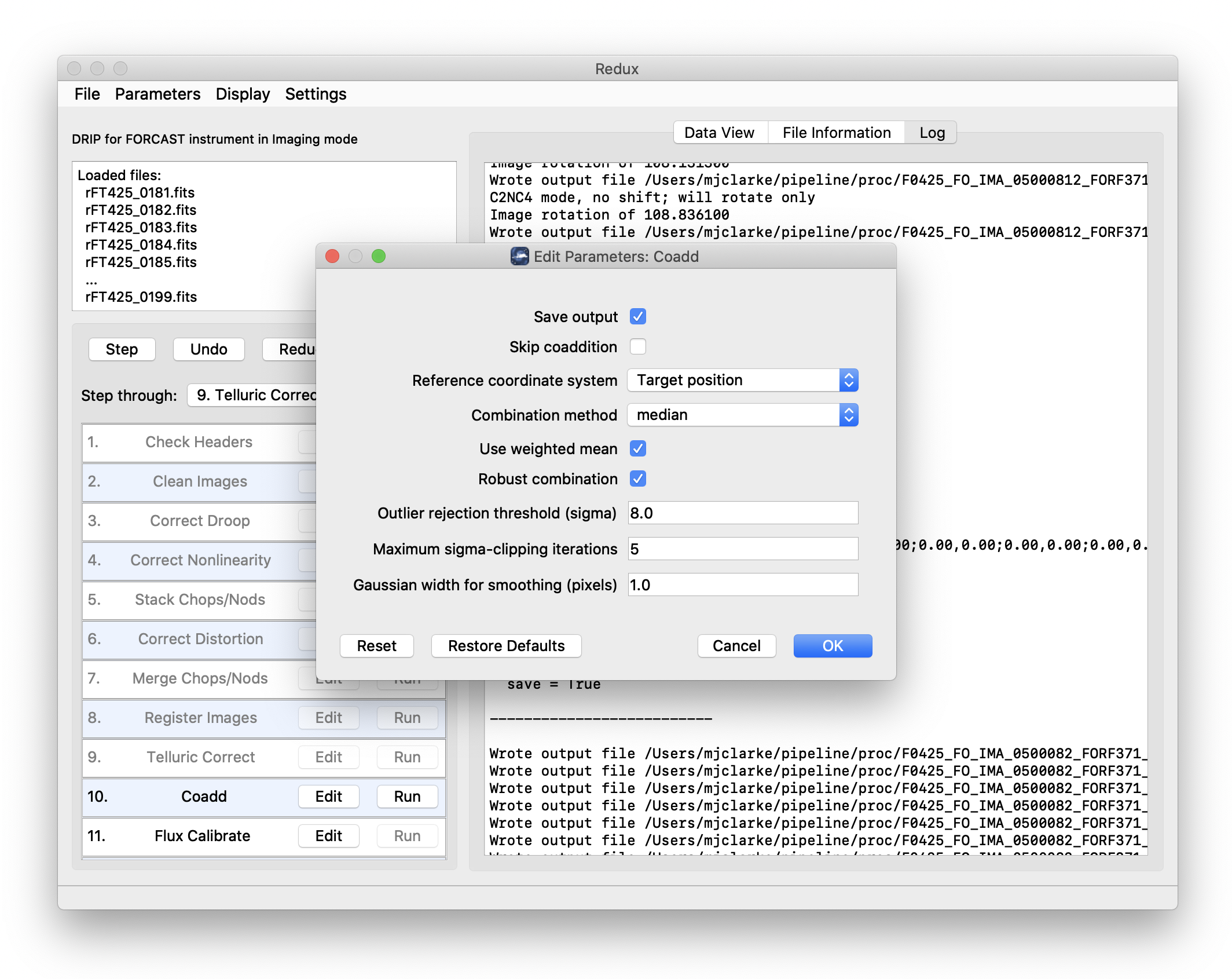
Fig. 89 Sample parameter editor for a pipeline step.

The current set of parameters can be displayed, saved to a file, or reset all at once using the Parameters menu. A previously saved set of parameters can also be restored for use with the current reduction (Parameters -> Load Parameters).

After all parameters for a step have been examined and set to the user’s satisfaction, a processing step can be run on all loaded files either by clicking Step, or the Run button next to the step name. Each processing step must be run in order, but if a processing step is selected in the Step through: widget, then clicking Step will treat all steps up through the selected step as a single step and run them all at once. When a step has been completed, its buttons will be grayed out and inaccessible. It is possible to undo one previous step by clicking Undo. All remaining steps can be run at once by clicking Reduce. After each step, the results of the processing may be displayed in a data viewer. After running a pipeline step or reduction, click Reset to restore the reduction to the initial state, without resetting parameter values.

Files can be added to the reduction set (File -> Add Files) or removed from the reduction set (File -> Remove Files), but either action will reset the reduction for all loaded files. Select the File Information tab to display a table of information about the currently loaded files (Fig. 90).

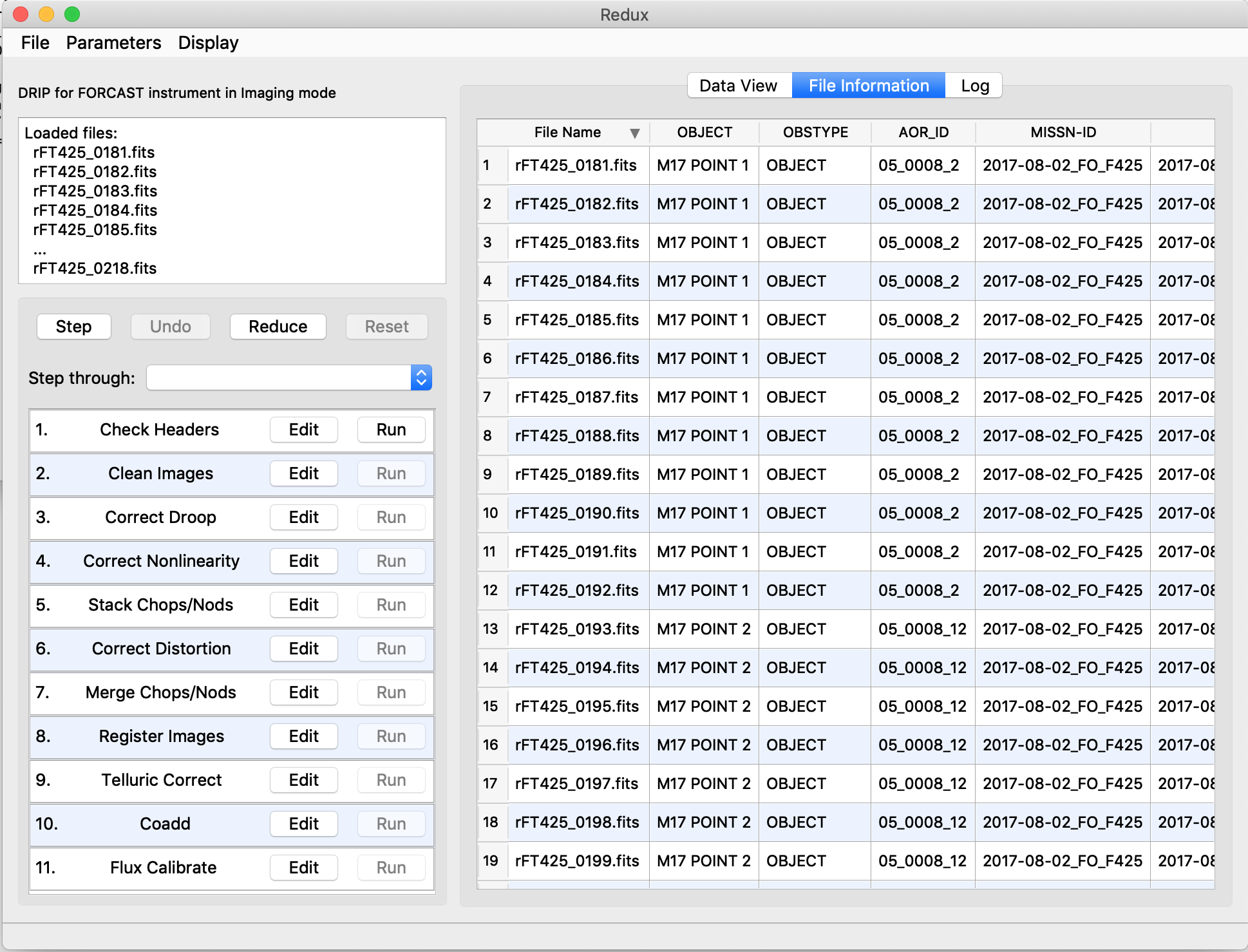
Fig. 90 File information table.

Display Features

The Redux GUI displays images for quality analysis and display (QAD) in the DS9 FITS viewer. DS9 is a standalone image display tool with an extensive feature set. See the SAO DS9 site (http://ds9.si.edu/) for more usage information.

After each pipeline step completes, Redux may load the produced images into DS9. Some display options may be customized directly in DS9; some commonly used options are accessible from the Redux interface, in the Data View tab (Fig. 91).

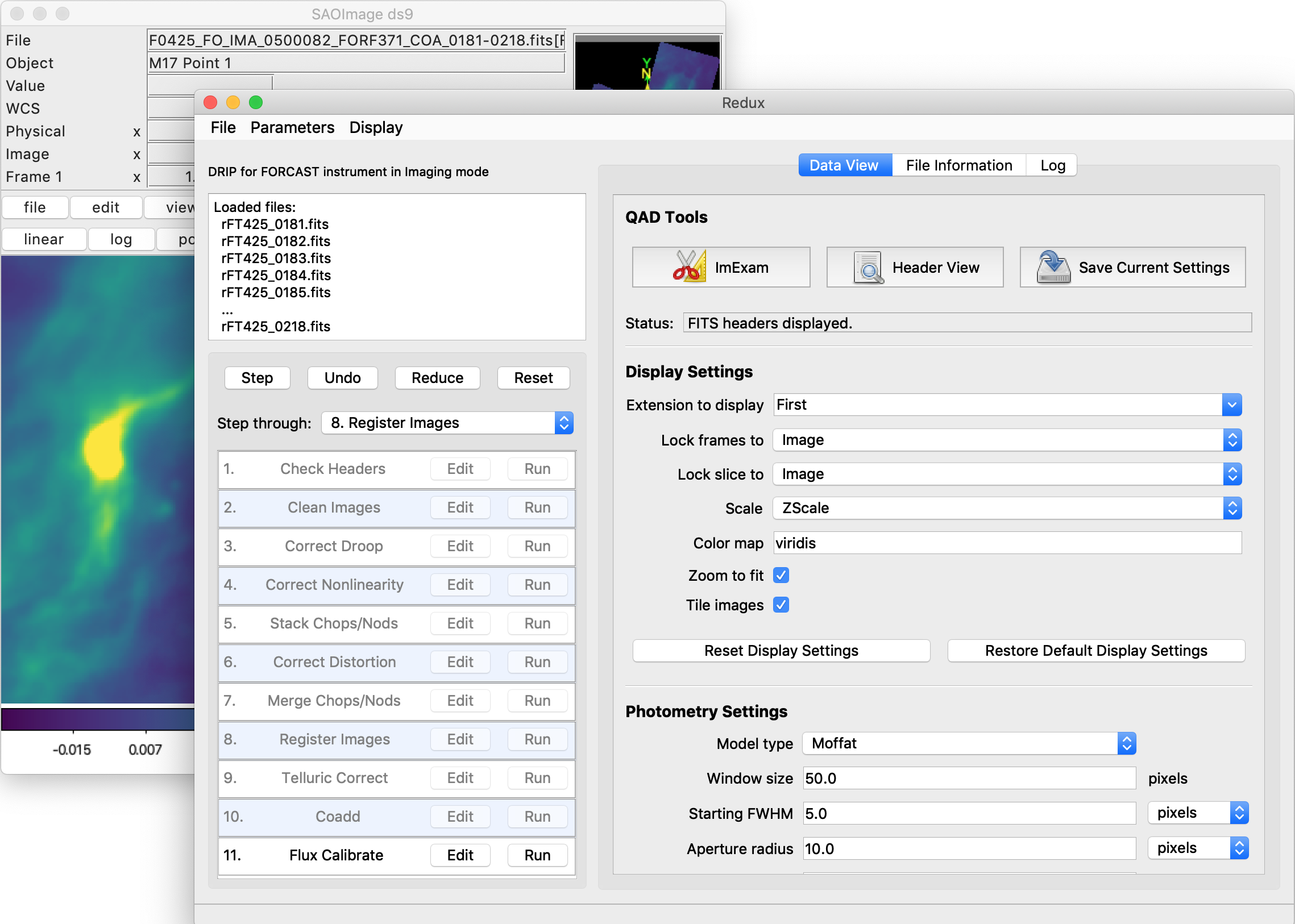
Fig. 91 Data viewer settings and tools.

From the Redux interface, the Display Settings can be used to:

• Set the FITS extension to display (First, or edit to enter a specific extension), or specify that all extensions should be displayed in a cube or in separate frames.

• Lock individual frames together, in image or WCS coordinates.

• Lock cube slices for separate frames together, in image or WCS coordinates.

• Set the image scaling scheme.

• Set a default color map.

• Zoom to fit image after loading.

• Tile image frames, rather than displaying a single frame at a time.

Changing any of these options in the Data View tab will cause the currently displayed data to be reloaded, with the new options. Clicking Reset Display Settings will revert any edited options to the last saved values. Clicking Restore Default Display Settings will revert all options to their default values.

In the QAD Tools section of the Data View tab, there are several additional tools available.

Clicking the ImExam button (scissors icon) launches an event loop in DS9. After launching it, bring the DS9 window forward, then use the keyboard to perform interactive analysis tasks:

• Type ‘a’ over a source in the image to perform photometry at the cursor location.

• Type ‘p’ to plot a pixel-to-pixel comparison of all frames at the cursor location.

• Type ‘s’ to compute statistics and plot a histogram of the data at the cursor location.

• Type ‘c’ to clear any previous photometry results or active plots.

• Type ‘h’ to print a help message.

• Type ‘q’ to quit the ImExam loop.

The photometry settings (the image window considered, the model fit, the aperture sizes, etc.) may be customized in the Photometry Settings. Plot settings (analysis window size, shared plot axes, etc.) may be customized in the Plot Settings. After modifying these settings, they will take effect only for new apertures or plots (use ‘c’ to clear old ones first). As for the display settings, the reset button will revert to the last saved values and the restore button will revert to default values. For the pixel-to-pixel and histogram plots, if the cursor is contained within a previously defined DS9 region (and the regions package is installed), the plot will consider only pixels within the region. Otherwise, a window around the cursor is used to generate the plot data. Setting the window to a blank value in the plot settings will use the entire image.

Clicking the Header button (magnifying glass icon) from the QAD Tools section opens a new window that displays headers from currently loaded FITS files in text form (Fig. 92). The extensions displayed depends on the extension setting selected (in Extension to Display). If a particular extension is selected, only that header will be displayed. If all extensions are selected (either for cube or multi-frame display), all extension headers will be displayed. The buttons at the bottom of the window may be used to find or filter the header text, or generate a table of header keywords. For filter or table display, a comma-separated list of keys may be entered in the text box.

Clicking the Save Current Settings button (disk icon) from the QAD Tools section saves all current display and photometry settings for the current user. This allows the user’s settings to persist across new Redux reductions, and to be loaded when Redux next starts up.

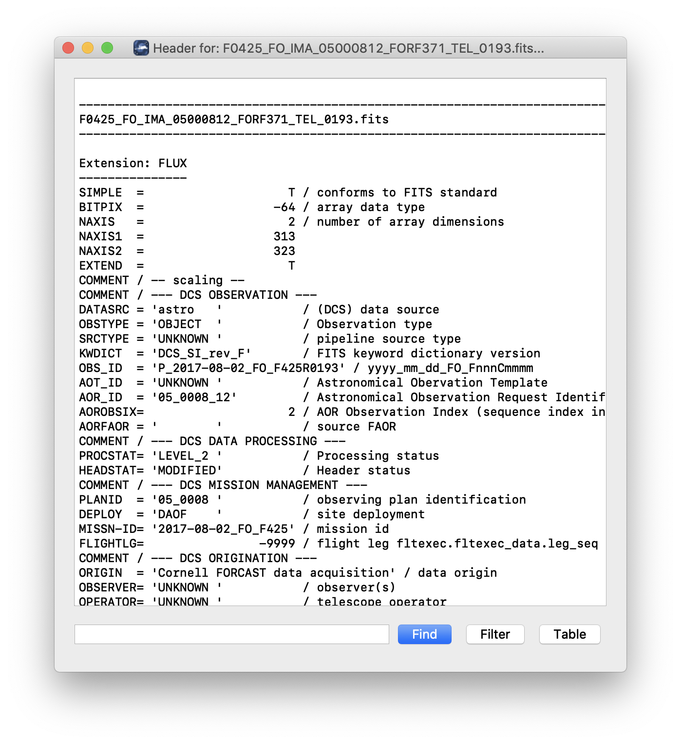
Fig. 92 QAD FITS header viewer.

FORCAST Reduction

Imaging Reduction

FORCAST imaging reduction with Redux is straightforward. The processing steps follow the flowchart of Fig. 77. At each step, Redux attempts to determine automatically the correct action, given the input data and default parameters, but each step can be customized as needed.

Useful Parameters

Some key parameters to note are listed below.

In addition to the specified parameters, the output from each step may be optionally saved by selecting the ‘save’ parameter.

• Check Headers

  • Abort reduction for invalid headers: By default, Redux will halt the reduction if the input header keywords do not meet requirements. Uncheck this box to attempt the reduction anyway.

• Clean Images

  • Bad pixel map: The default bad pixel mask on disk is automatically loaded. Set blank to use no bad pixel map. Set to a valid FITS file path to override the default bad pixel mask with a new one.

  • Automatically detect readout shift: If selected, the pipeline will attempt to automatically detect and correct the readout shift described below.

  • Image number to shift (if not auto): This option allows the user to fix an occasional issue where the data array is shifted to the right by 16 pixels. If multiple images are loaded, but only some are affected, the images to shift may be specified by their index in the list of input files, separated by semi-colons. For example, to shift the first and third file, enter ‘1;3’. If all input files should be shifted, enter ‘all’. Leave blank to leave all data unshifted (the default behavior).

  • Interpolate over bad pixels: By default, bad pixels are propagated as NaN values. Set this option to interpolate over them instead.

• Correct Droop

  • Droop fraction: Lower value to decrease droop correction; set to zero to turn off droop correction altogether. Default value is currently 0.0035 for all data.

• Correct Nonlinearity

  • Background section center: Specify the center point of the region used to determine the background level in integers as ‘x,y’, in pixels.

  • Background section size: Specify the width of the background region in integer pixels as ‘size_x,size_y’.

• Stack Chops/Nods

  • Add all frames instead of subtracting: If set, the instrument mode will be ignored and all chops and nods will be added. This option may be used to generate a sky frame, for debugging or calibration purposes.

  • Apply ‘jailbar’ correction: If set, the 16-pixel jailbar pattern will be removed after stacking.

  • Scale frames to common level: If selected, images will be corrected for a multiplicative offset in the background level. This is not commonly used.

  • Subtract residual background: If selected, images will be corrected for an additive offset in the background level. This option is off by default for C2NC2 data, but on for all other modes. Background differences may occasionally be overcorrected, in which case, this option should be deselected, or the background section modified. Some C2NC2 data with sufficient background regions may also benefit from turning this option on.

  • Background section center: Specify the center point of the region used to determine the background level in integers as ‘x,y’, in pixels.

  • Background section size: Specify the width of the background region in integer pixels as ‘size_x,size_y’.

  • Residual background statistic: Select the statistic used to calculate the background level. Options are median or mode.

• Correct Distortion

  • Pinhole locations: The default pinhole mask table is automatically loaded. Set to a valid text file path to override it.

  • Skip distortion: This option allows one to skip distortion correction.

  • Extrapolate solution: If not set, edges of the image beyond known pinhole inputs will be set to NaN.

• Merge Chops/Nods

  • Merging algorithm: The default for flux standard observations (OBSTYPE=STANDARD_FLUX) is to shift-and-add the data, using a centroiding algorithm. If the centroiding algorithm fails, header data will be used instead. The default for science data is not to shift-and-add (‘No shift’).

  • Skip rotation: If set, the sky angle rotation correction is not applied to both the image and the WCS coordinate system.

• Register Images

  • Registration algorithm: The default for all data is to use the WCS as is for registration. Centroiding is may be useful for bright, compact objects; cross-correlation may be useful for bright, diffuse fields. Registration via the ‘Header shifts’ method may be useful for older data, for which the relative WCS is not very accurate. The ‘Use first WCS’ option will treat all images as pre-registered: the data will be coadded directly without shifts.

  • Override offsets for all images: If registration offsets are known a priori, they may be directly entered here. Specify semi-colon separated offsets, as x,y. For example, for three input images, specify ‘0,0;2,0;0,2’ to leave the first as is, shift the second two pixels to the right in x, and shift the third two pixels up in y.

  • Expected FWHM for centroiding: Specify the expected FWHM in pixels, for the centroiding algorithm. This may be useful in registering bright compact sources that are not point sources.

  • Maximum shift for cross-correlation: Specify the maximum allowed shift in pixels for the cross-correlation algorithm. This limit is applied for shifts in both x- and y-direction.

• Telluric Correct

  • Use WV values: If set, water vapor values from the header (WVZ_OBS) will be used to correct for atmospheric transmission, instead of altitude.

• Coadd

  • Skip coaddition: If selected, each input registered file will be saved as a separate file of type ‘coadded’ rather than combined together into a single output file.

  • Reference coordinate system: If set to ‘First image’, all images will be referenced to the sky position in the first image file. If set to ‘Target position’, the TGTRA/TGTDEC keywords in the FITS header will be used to apply an additional offset for registering non-sidereal targets. If these keywords are not present, or if their value is constant, the algorithm defaults to the ‘First image’ behavior. ‘Target position’ is on by default; ‘First image’ is recommended only if the TGTRA/TGTDEC keywords are known to have bad values.

  • Combination method: Median is the default; mean may also be useful for some input data. The resample option may project data more accurately, and allows an additional smoothing option, but takes much longer to complete.

  • Use weighted mean: If set, the average of the data will be weighted by the variance. Ignored for method=median.

  • Robust combination: If set, data will be sigma-clipped before combination for mean or median methods.

  • Outlier rejection threshold (sigma): The sigma-clipping threshold for robust combination methods, in units of sigma (standard deviation).

  • Gaussian width for smoothing (pixels): If method=resample, a smoothing may be applied to the output averages. Specify the Gaussian width in pixels. Set smaller (but non-zero) for less smoothing; higher for more smoothing.

• Flux Calibrate

  • Re-run photometry for standards: If selected, and observation is a flux standard, photometric fits and aperture measurements on the brightest source will be recalculated, using the input parameters below.

  • Source position: Enter the approximate position (x,y) of the source to measure. If not specified, the SRCPOSX/SRCPOSY keywords in the FITS header will be used as the first estimate of the source position.

  • Photometry fit size: Smaller subimages may sometimes be necessary for faint sources and/or variable background.

  • Initial FWHM: Specify in pixels. This parameter should be modified only if the PSF of the source is significantly larger or smaller than usual.

  • Profile type: Moffat fits are the default, as they generally give a more reliable FWHM value. However, Gaussian fits may sometimes be more stable, and therefore preferable if the Moffat fit fails.

• Make Image Map

  • Color map: Color map for the output PNG image. Any valid Matplotlib name may be specified.

  • Flux scale for image: A low and high percentile value , used for scaling the image, e.g. [0,99].

  • Number of contours: Number of contour levels to be over-plotted on the image. Set to 0 to turn off contours.

  • Contour color: Color for the contour lines. Any valid Matplotlib color name may be specified.

  • Filled contours: If set, contours will be filled instead of overlaid.

  • Overlay grid: If set, a coordinate grid will be overlaid.

  • Beam marker: If set, a beam marker will be added to the plot.

  • Watermark text: If set to a non-empty string, the text will be added to the lower-right of the image as a semi-transparent watermark.

  • Crop NaN border: If set, any remaining NaN or zero-valued border will be cropped out of plot.

Grism Reduction

Spectral extraction with Redux is slightly more complicated than image processing. The GUI breaks down the spectral extraction algorithms into six separate reduction steps to give more control over the extraction process. These steps are:

• Make Profiles: Generate a smoothed model of the relative distribution of the flux across the slit (the spatial profile). After this step is run, a separate display window showing a plot of the spatial profile appears.

• Locate Apertures: Use the spatial profile to identify spectra to extract. By default, Redux attempts to automatically identify sources, but they can also be manually identified by entering a guess position to fit near, or a fixed position, in the parameters. Aperture locations are plotted in the profile window.

• Trace Continuum: Identify the location of the spectrum across the array, by either fitting the continuum or fixing the location to the aperture center. The aperture trace is displayed as a region overlay in DS9.

• Set Apertures: Identify the data to extract from the spatial profile. This is done automatically by default, but all aperture parameters can be overridden manually in the parameters for this step. Aperture radii and background regions are plotted in the profile window (see Fig. 93).

• Subtract Background: Residual background is fit and removed for each column in the 2D image, using background regions specified in the Set Apertures step.

• Extract Spectra: Extract one-dimensional spectra from the identified apertures. By default, Redux will perform standard extraction for observations that are marked as extended sources (SRCTYPE=EXTENDED_SOURCE) and will attempt optimal extraction for any other value. The method can be overridden in the parameters for this step.

Extracted spectra are displayed in an interactive plot window, for data analysis and visualization (see Fig. 94).

The spectral display tool has a number of useful features and controls. See Fig. 95 and the table below for a quick summary.

Table 23 Spectral Viewer controls

Feature	Control	Keyboard shortcut
Load new FITS file	File Choice -> Add File	–
Remove loaded FITS file	File Choice -> Remove File	Press delete in the File Choice panel
Plot selected file	File Choice -> (double-click)	–
Add a new plot window (pane)	Panes -> Add Pane	–
Remove a pane	Panes -> Remove Pane	Press delete in the Panes panel, or in the plot window
Show or hide a plot	Panes -> Pane # -> File name -> Enabled, or click the Hide all/ Show all button	–
Display a different X or Y field (e.g. spectral error, transmission, or response)	Axis -> X Property or Y Property	–
Overplot a different Y axis field (e.g. spectral error, transmission, or response)	Axis -> Overplot -> Enabled	–
Change X or Y units	Axis -> X Unit or Y Unit	–
Change X or Y scale	Axis -> X Scale or Y Scale -> Linear or Log	–
Interactive zoom	Axis -> Zoom: X, Y, Box, then click in the plot to set the limits; or Reset to reset the limits to default.	In the plot window, press x, y, or z to start zoom mode in x-direction, y-direction, or box mode, respectively. Click twice on the plot to set the new limits. Press w to reset the plot limits to defaults.
Fit a spectral feature	–	In the plot window, press f to start the fitting mode. Click twice on the plot to set the data limits to fit.
Change the feature or baseline fit model	Analysis -> Feature, Background	–
Load a spectral line list for overplot display	Analysis -> Reference Data: Open, Load List Select a one- or two- column text file containing wavelengths in microns and (optionally) labels for the values. Columns may be comma, space, or ‘|’ separated.	–
Clear zoom or fit mode	–	In the plot window, press c to clear guides and return to default display mode.
Change the plot color cycle	Plot -> Color cycle -> Accessible, Spectral or Tableau	–
Change the plot type	Plot -> Plot type -> Step, Line, or Scatter	–
Change the plot display options	Plot -> Show markers, Show errors, Show grid, or Dark mode	–
Display the cursor position	Cursor panel -> Check Cursor Location for a quick display or press Popout for full information	–

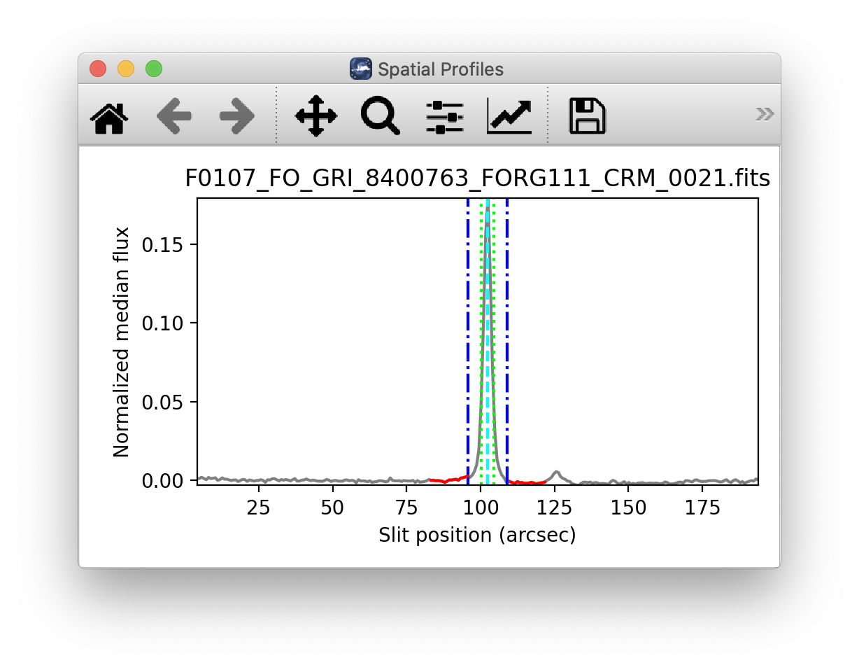
Fig. 93 Aperture location automatically identified and over-plotted on the spatial profile. The cyan line indicates the aperture center. Green lines indicate the integration aperture for optimal extraction, dark blue lines indicate the PSF radius (the point at which the flux goes to zero), and red lines indicate background regions.

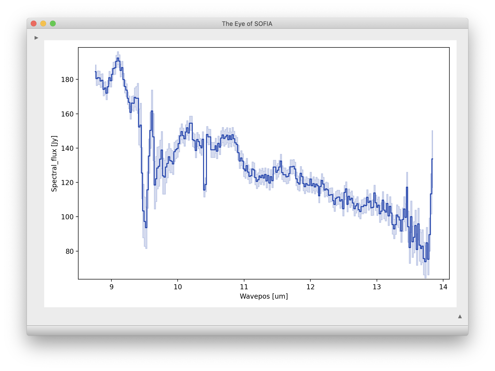
Fig. 94 Final extracted spectrum, displayed in an interactive plot window.

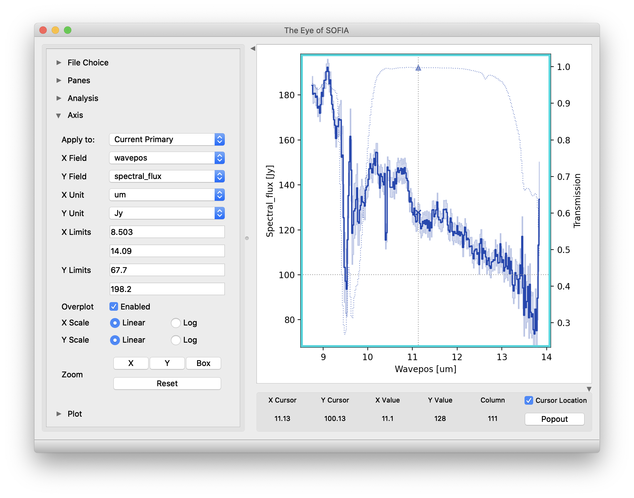
Fig. 95 Control panels for the spectral viewer are located to the left and below the plot window. Click the arrow icons to show or collapse them.

Useful Parameters

Below are listed some key parameters for the grism processing steps. Note that the Check Headers through Stack Chops/Nods steps are identical to those used for the imaging data: their parameters are listed above. In addition to the specified parameters, the output from each step may be optionally saved by selecting the ‘save’ parameter.

• Stack Dithers

  • Skip dither stacking: If set, common dither positions will not be stacked. This is the default: dither stacking is only recommended for faint spectra that cannot otherwise be automatically extracted.

  • Ignore dither information from header: If set, all input files are stacked regardless of dither position.

  • Combination method: Mean is the default; median may also be useful for some input data.

  • Use weighted mean: If set, the average of the data will be weighted by the variance. Ignored for method=median.

  • Robust combination: If set, data will be sigma-clipped before combination.

  • Outlier rejection threshold (sigma): The sigma-clipping threshold for robust combination methods, in units of sigma (standard deviation).

• Make Profiles

  • Wave/space calibration file: The default calibration file is automatically loaded. Set to a valid FITS file path to override the default calibration map with a new one.

  • Slit correction file: The default slit correction file is automatically loaded, if available. If blank, no slit correction will be applied. Set to a valid FITS file path to override the default file with a new one.

  • Row fit order: Typically a third-order polynomial fit is used to calculate the smooth spatial profile. Occasionally, a higher or lower order fit may give better results.

  • Subtract median background: If set, then the median level of the smoothed spatial profile will be subtracted out to remove residual background from the total extracted flux. If the SRCTYPE is EXTENDED_SOURCE or the INSTMODE is slitscan, this option will be off by default. For other data, this option is appropriate as long as the slit is dominated by background, rather than source flux. If the spatial profile dips below zero at any point (other than for a negative spectrum), this option should be deselected.

  • Atmospheric transmission threshold: Transmission values below this threshold are not considered when making the spatial profile. Values are 0-1.

  • Simulate calibrations: Simulate calibration values instead of using the wave/space calibration file. This option is primarily used for testing.

• Locate Apertures

  • Aperture location method: If ‘auto’, the strongest Gaussian peak(s) in the spatial profile will be selected, with an optional starting guess (Aperture position, below). If ‘fix to input’, the value in the Aperture position parameter will be used without refinement. If ‘fix to center’, the center of the slit will be used. ‘Fix to center’ is default for EXTENDED_SOURCE and SLITSCAN; otherwise ‘auto’ is default.

  • Number of auto apertures: Set this parameter to 1 to automatically find the single brightest source, or 2 to find the two brightest sources, etc. Sources may be positive or negative.

  • Aperture position: Enter a guess value for the aperture to use as a starting point for method = ‘auto’, or a fixed value to use as the aperture center for method = ‘fix to input’. Values are in arcseconds up the slit (refer to the spatial profile). Separate multiple apertures for a single file by commas; separate values for multiple files by semi-colons. For example, 3,8;2,7 will look for two apertures in each of two files, near 3” and 8” in the first image and 2” and 7” in the second image. If there are multiple files loaded, but only one aperture list is given, the aperture parameters will be used for all images.

  • Expected aperture FWHM (arcsec): Gaussian FWHM estimate for spatial profile fits, to determine peaks.

• Trace Continuum

  • Trace method: If ‘fit to continuum’ is selected, points along the continuum will be fit with a Gaussian to determine the trace center at each location, and then the positions will be fit with a low-order polynomial. If ‘fix to aperture position’ is selected, no fit will be attempted, and the default slit curvature defined by the edge definition file will be used as the aperture location. By default, the trace will be fixed for EXTENDED_SOURCE and SLITSCAN, but a fit will be attempted for all other data types.

  • Trace fit order: Polynomial fit order for the aperture center, along the spectral dimension.

• Set Apertures

  • Extract the full slit: If set, all other parameters are ignored, and the PSF radius will be set to include the full slit.

  • Refit apertures for FWHM: The spatial FWHM for the aperture is used to determine the aperture and PSF radii, unless they are directly specified. If this parameter is set, the profile will be re-fit with a Gaussian to determine the FWHM. If it is not set, the value determined or set in the Locate Apertures step is used (stored as APFWHM01 in the FITS header).

  • Aperture sign: Enter either 1 or -1 to skip the automatic determination of the aperture sign from the spatial profile. If the value is -1, the spectrum will be multiplied by -1. Separate multiple apertures by commas; separate values for multiple files by semi-colons. If a single value is specified, it will be applied to all apertures.

  • Aperture radius: Enter a radius in arcsec to skip the automatic determination of the aperture radius from the profile FWHM. Separate multiple apertures by commas; separate values for multiple files by semi-colons. If a single value is specified, it will be applied to all apertures.

  • PSF radius: Enter a radius in arcsec to skip the automatic determination of the PSF radius from the profile FWHM. Separate multiple apertures by commas; separate values for multiple files by semi-colons. If a single value is specified, it will be applied to all apertures.

  • Background regions: Enter a range in arcsec to use as the background region, skipping automatic background determination. For example, 0-1,8-10 will use the regions between 0” and 1” and between 8” and 10” to determine the background level to subtract in extraction. Values are for the full image, rather than for a particular aperture. Separate values for multiple files with semi-colons.

• Subtract Background

  • Skip background subtraction: Set to skip calculating and removing residual background. If no background regions were set, background subtraction will be automatically skipped.

  • Background fit order: Set to a number greater than or equal to zero for the polynomial order of the fit to the background regions.

• Extract Spectra

  • Save extracted 1D spectra: If set, the extracted spectra will be saved to disk in Spextool format. This option is normally used only for diagnostic purposes.

  • Extraction method: The default is to use standard extraction for EXTENDED_SOURCE and SLITSCAN and optimal extraction otherwise. Standard extraction may be necessary for some faint sources.

  • Use median profile instead of spatial map: By default, the pipeline uses a wavelength-dependent spatial map for extraction, but this method may give poor results, if the signal-to-noise in the profile is low. Set this option to use the median spatial profile across all wavelengths instead.

  • Use spatial profile to fix bad pixels: The pipeline usually uses the spatial profile to attempt to fix bad pixels during standard extraction, and in the 2D image for either extraction method. Occasionally, this results in a failed extraction. Unset this options to extract the spectra without bad pixel correction.

  • Bad pixel threshold: Enter a value for the threshold for a pixel to be considered a bad pixel. This value is multiplied by the standard deviation of all good pixels in the aperture at each wavelength bin.

• Merge Apertures

  • Save uncalibrated 1D spectra: If set, the merged spectra will be saved to disk in Spextool format. This option is normally used only for diagnostic purposes.

  • Combination method: Mean is the default; median may also be useful for some input data.

  • Use weighted mean: If set, the average of the data will be weighted by the variance. Ignored for method=median.

• Flux Calibrate

  • General Parameters

    • Save calibrated 1D spectra: If set, the calibrated spectra will be saved to disk in Spextool format. This option is normally used only for diagnostic purposes.

    • Skip flux calibration: If set, no telluric correction or flux calibration will be applied.

    • Response file: The default instrumental response file on disk is automatically loaded. If blank, no response correction will be applied, but transmission correction will still occur. Set to a valid FITS file path to override the default response file with a new one.

    • Spectral resolution: Expected resolution for the grism mode, used to smooth the ATRAN model. This value should match that of the response file, and should only need modification if the response file is modified from the default.

  • Telluric Correction Parameters

    • Optimize ATRAN correction: If set, the pipeline will use a library of ATRAN files to attempt to automatically select the best telluric correction. This option requires that the external library location be identified in the ATRAN directory parameter. The procedure may take some time to complete, and may not complete successfully for faint spectra, or spectra with significant emission features. Optimization will not be attempted for the FOR_G111 grism, or for spectra with mean S/N less than the specified threshold.

    • ATRAN directory: This parameter specifies the location of the library of ATRAN FITS files to use. If blank, the default files provided with the pipeline will be used. If optimization is desired, this library must contain files parameterized by PWV.

    • ATRAN file: This parameter is used to override the ATRAN file to use for telluric correction. If blank, the default ATRAN file on disk will be used. Set to a valid FITS file path to override the default ATRAN file with a new one.

    • Use WV values: If set, and optimize is not set, water vapor values from the header (WVZ_OBS) will be used to choose the correct ATRAN file.

    • S/N threshold for optimization: If the median S/N for a spectrum is below this threshold, optimization will not be attempted. Automatic wavelength shifts will also not be attempted.

  • Wavelength Shift Parameters

    • Auto shift wavelength to telluric spectrum: If set, the data will be shifted to match the telluric spectrum. The optimum shift chosen is the one that minimizes residuals in the corrected spectrum, when fit with a low order polynomial. All values within the range of the maximum shift are tested, at a resolution of 0.1 pixels. Auto shift will not be attempted for the FOR_G111 grism.

    • Maximum auto wavelength shift to apply: The maximum shift allowable for auto-shifts, in pixels.

    • Wavelength shift to apply: Set to specify a manual shift in pixels along the wavelength axis to apply to the science spectrum. If non-zero, the auto-shift parameter will be ignored.

    • Polynomial order for continuum: The fit order for the spectrum, used to determine the optimum wavelength shift.

• Combine Spectra

  • General Parameters

    • Registration method: If set to ‘Use WCS as is’, all images will be referenced to the sky position in the first image file. If set to ‘Correct to target position’, the TGTRA/TGTDEC keywords in the FITS header will be used to apply an additional offset for registering non-sidereal targets. If these keywords are not present, or if their value is constant, the algorithm defaults to the ‘Use WCS as is’ behavior. ‘Correct to target position’ is on by default; the other options are recommended only if the TGTRA/TGTDEC or WCS keywords are known to have bad values. In that case, set to ‘Use header offsets’ for non-sidereal targets or files with known bad WCS parameters; otherwise use ‘Use WCS as is’.

    • Combination method: Mean is the default for all data not marked SLITSCAN; median may also be useful for some input data. For SLITSCAN, the default is ‘spectral cube’. If this option is set, the input data will be resampled into a 3D spatial/spectral cube instead of coadding 1D spectra and 2D images.

    • Weight by errors: If set, the average of the data will be weighted by the errors. Ignored for method=median.

  • 1-2D Combination Parameters

    • Robust combination: If set, data will be sigma-clipped before combination for mean or median methods.

    • Outlier rejection threshold (sigma): The sigma-clipping threshold for robust combination methods, in units of sigma (standard deviation).

  • 3D Resample Parameters

    • Spatial surface fit order: This parameter controls the polynomial order of the surface fit to the data at each grid point. Higher orders give more fine-scale detail, but are more likely to be unstable. Set to zero to do a weighted mean of the nearby data.

    • Spatial fit window: Spatial window (pixels) for consideration in local data fits. Set higher to fit to more pixels.

    • Spatial smoothing radius: Gaussian width (pixels) for smoothing radius in distance weights for local data fits. Set higher to smooth over more pixels.

    • Spatial edge threshold: A value between 0 and 1 that determines how much of the image edge is set to NaN. Set higher to set more pixels to NaN.

    • Adaptive smoothing algorithm: If ‘scaled’, the size of the smoothing kernel is allowed to vary, in order to optimize reconstruction of sharply peaked sources. If ‘shaped’, the kernel shape and rotation may also vary. If ‘none’, the kernel will not vary.

• Make Spectral Map

  • Color map: Color map for the output PNG image. Any valid Matplotlib name may be specified.

  • Flux scale for image: A low and high percentile value , used for scaling the spectral image, e.g. [0,99].

  • Number of contours: Number of contour levels to be over-plotted on the image. Set to 0 to turn off contours.

  • Contour color: Color for the contour lines. Any valid Matplotlib color name may be specified.

  • Filled contours: If set, contours will be filled instead of overlaid.

  • Overlay grid: If set, a coordinate grid will be overlaid.

  • Watermark text: If set to a non-empty string, the text will be added to the lower-right of the image as a semi-transparent watermark.

  • Fraction of outer wavelengths to ignore: Used to block edge effects for noisy spectral orders. Set to 0 to include all wavelengths in the plot.

  • Overplot transmission: If set, the atmospheric transmission spectrum will be displayed in the spectral plot.

  • Flux scale for spectral plot: Specify a low and high percentile value for the spectral flux scale, e.g. [0,99]. If set to [0, 100], Matplotlib defaults are used.

  • Override wavelength slice for spectral cube: Manually specify the wavelength slice (zero-indexed) for the image. Otherwise, the peak voxel in the cube is used to identify the spectral slice.

  • Override spatial point for spectral cube: Manually specify the spatial index for the spectrum, as ‘x,y’, zero-indexed. Otherwise, the peak voxel in the cube is used to identify the spatial point.

• Make Response

  • Standard model file: If blank, a model file will be searched for in the default data directory. Set to a valid FITS file to override.

Data Quality Assessment

After the pipeline has been run on a set of input data, the output products should be checked to ensure that the data has been properly reduced. Data quality and quirks can vary widely across individual observations, but the following general guideline gives some strategies for approaching quality assessment (QA) for FORCAST data.

• Check for QA comments in the FITS header HISTORY. These comments may make suggestions for files to exclude from final reductions, or for non-default parameters to set for optimal reductions.

• Check the output to the log file (usually called redux_[date]_[time].log), written to the same directory as the output files. Look for messages marked ERROR or WARNING. The log will also list every parameter used in the pipeline steps, which may help disambiguate the parameters as actually-run for the pipeline.

• Check that the expected files were written to disk: there should, at a minimum, be a calibrated file (CAL) for imaging data and a combined spectrum (CMB) for grism data. Check the data product tables (Table 15 and Table 16) for other expected data products for each mode.

• For imaging:

  • If shifting-and-adding was performed at the merge step, display all undistorted (UND) and merged (MRG) files. Check that the pattern of positive and negative sources looks right for the observation mode. Also check that the FWHM of the source is not worse in the merged files than it was in the undistorted files. If the pattern does not look right, or the FWHM is too large, the merge may have failed.

  • Display all registered and telluric-corrected (TEL) files at once and check that any visible sources appear at the same WCS coordinates in all files.

  • Display the final coadded (COA) or calibrated (CAL) file and check that the FWHM is not worse than it is in the registered files, which might indicate poor registration. Check for any unusual artifacts, such as variable background regions, or detector pattern noise.

  • Compare the calculated reference calibration factors for all flux standards to the last known series average. Major deviations may indicate that the photometry failed for that observation.

• For grism:

  • Display the spatial profile with apertures overlaid. Verify that apertures look well placed and the spatial profile does not dip below zero (except for negative spectral traces).

  • Display the rectified image, and overlay the locations of the extracted apertures. Verify that the apertures lie on top of any visible spectral traces.

  • Display the final spectrum (CMB) and overplot the expected atmospheric transmission. Check that the calibrated spectrum does not include residual artifacts from the telluric absorption features. If it does, the assumed resolution for the grism, or the wavelength calibration of the observation, may need updating.

  • Overlay a model spectrum on the calibrated spectra of flux standards. Verify that the observed spectrum matches the theoretical spectrum, within the error bars of the observation. If it does not, the instrumental response file may need updating.

Appendix A: Sample configuration files

Below are sample FORCAST Redux parameter override files in INI format. If present, the parameter value overrides the default defined by the FORCAST reduction object. If not present, the default value will be used.

# Redux parameters for FORCAST instrument in Imaging mode
# Pipeline: FORCAST_REDUX v2_3_0
[1: checkhead]
    abort = True
[2: clean]
    save = False
    badfile = lwc_badpix_OC7D.fits
    autoshift = True
    shiftfile = ""
    interpolate = False
[3: droop]
    save = False
    fracdroop = 0.0035
[4: nonlin]
    save = False
    secctr = "128,128"
    secsize = "190,190"
[5: stack]
    save = False
    add_frames = False
    jbclean = True
    bgscale = False
    bgsub = True
    secctr = "128,128"
    secsize = "190,190"
    bgstat = median
[6: undistort]
    save = True
    pinfile = pinhole_locs_LWC_20190629.txt
    transform_type = polynomial
    extrapolate = True
[7: merge]
    save = True
    cormerge = Centroid
[8: register]
    save = False
    corcoadd = Use WCS as is
    offsets = ""
    mfwhm = 4.5
    xyshift = 40.0
[9: tellcor]
    save = True
[10: coadd]
    save = True
    skip_coadd = False
    reference = Target position
    method = median
    weighted = True
    robust = True
    threshold = 8.0
    maxiters = 5
    smoothing = 1.0
[11: fluxcal]
    save = True
    rerun_phot = False
    srcpos = ""
    fitsize = 138
    fwhm = 5.0
    profile = Moffat
[12: imgmap]
    colormap = plasma
    scale = 0.25, 99.9
    n_contour = 0
    contour_color = gray
    fill_contours = False
    grid = False
    beam = True
    watermark = ""
    crop_border = True

# Redux parameters for FORCAST instrument in Spectroscopy mode
# Pipeline: FORCAST_REDUX v2_3_0
[1: checkhead]
    abort = True
[2: clean]
    save = False
    badfile = swc_badpix_OC2.fits
    autoshift = True
    shiftfile = ""
    interpolate = False
[3: droop]
    save = False
    fracdroop = 0.0035
[4: nonlin]
    save = False
    secctr = "128,128"
    secsize = "190,190"
[5: stack]
    save = True
    add_frames = False
    jbclean = True
    bgscale = False
    bgsub = False
    secctr = "128,128"
    secsize = "190,190"
    bgstat = median
[6: stack_dithers]
    save = True
    skip_stack = True
    ignore_dither = False
    method = mean
    weighted = True
    robust = True
    threshold = 8.0
    maxiters = 5
[7: make_profiles]
    save = True
    wavefile = G063_wavecal_OC2.fits
    slitfile = G063_LS24_slitfn_OC2.fits
    fit_order = 3
    bg_sub = True
    atmosthresh = 0.0
    simwavecal = False
[8: locate_apertures]
    save = False
    method = auto
    num_aps = 1
    input_position = ""
    fwhm = 3.0
[9: trace_continuum]
    save = False
    method = fit to continuum
    fit_order = 2
[10: set_apertures]
    save = False
    full_slit = False
    refit = True
    apsign = ""
    aprad = ""
    psfrad = ""
    bgr = ""
[11: subtract_background]
    save = False
    skip_bg = False
    bg_fit_order = 0
[12: extract_spectra]
    save = False
    save_1d = False
    method = optimal
    use_profile = False
    fix_bad = True
    threshold = 10.0
[13: merge_apertures]
    save = True
    save_1d = False
    method = mean
    weighted = True
[14: flux_calibrate]
    save = True
    save_1d = False
    skip_cal = False
    respfile = G063_LS24_DB175_response.fits
    resolution = 180.0
    optimize_atran = True
    atrandir = $DPS_SHARE/calibrations/ATRAN/fits
    atranfile = ""
    sn_threshold = 10.0
    auto_shift = True
    auto_shift_limit = 2.0
    waveshift = 0.0
    model_order = 1
[15: combine_spectra]
    save = True
    registration = Correct to target position
    method = mean
    weighted = True
    robust = True
    threshold = 8.0
    maxiters = 5
    fit_order = 2
    fit_window = 7.0
    smoothing = 2.0
    edge_threshold = 0.7
    adaptive_algorithm = none
[16: specmap]
    colormap = plasma
    scale = 0.25, 99.9
    n_contour = 0
    contour_color = gray
    fill_contours = False
    grid = False
    watermark = ""
    ignore_outer = 0.0
    atran_plot = True
    spec_scale = 0, 100
    override_slice = ""
    override_point = ""

Appendix B: Required input keywords

This table describes the type and expected value for all FITS keywords used by the FORCAST pipeline.

Table 24 Required input keywords

Keyword	Type	Expected value
ALTI_STA	float	0-60000.
ALTI_END	float	0-60000.
AOR_ID	string
DATASRC	string	ASTRO, CALIBRATION, LAB, TEST, OTHER, FIRSTPOINT
DATE-OBS	string	yyyy-mm-ddThh:mm:ss[.sss]
DETCHAN	string	SW, LW
DETECTOR	string	As-010, Sb-083
DETITIME	float	> 0
EPERADU	float	> 1
FRMRATE	float	> 0
ILOWCAP	bool
INSTCFG	string	IMAGING_SWC, IMAGING_LWC, IMAGING_DUAL, GRISM_XD, GRISM_SWC, GRISM_LWC, GRISM_DUAL, GRISM_XD-LSV, GRISM-SSV, GRISM-LSV
INSTMODE	string	C2, C2N, C2NC2, N, SLITSCAN, NXCAC
INSTRUME	string	FORCAST
INTTIME	float
MISSN_ID	string
NAXIS1	int	256
NAXIS2	int	256
OBJECT	string
OBS_ID	string
OBSTYPE	string	OBJECT, STANDARD_FLUX, STANDARD_TELLURIC, LAMP, FLAT, DARK, BIAS, SKY, BB, GASCELL, LASER, FOCUS_LOOP
OTMODE	string	AD, SUR
OTSTACKS	int	>0
SPECTEL1	string	NONE, FOR_F054, FOR_F064, FOR_F066, FOR_F077, FOR_F111, FOR_F113, FOR_F197, FOR_F253, FOR_XG063, FOR_XG111, FOR_G063, FOR_G111
SPECTEL2	string	NONE, FOR_F086, FOR_F113, FOR_F118, FOR_F254, FOR_F315, FOR_F336, FOR_F348, FOR_F371, FOR_F242, FOR_G227, FOR_G329
TELESCOP	string	SOFIA
TIME-OBS	string
UTCSTART	string
WAVELNTH	float	0-40.
ZA_START	float	0-90.
ZA_END	float	0-90.
DITHER	bool
DTHCRSYS	string	SIRF, ERF
DTHINDEX	int	> 0
DITHERX	float
DITHERY	float
CHOPPING	bool
CHPCRSYS	string	SIRF, ERF
CHPAMP1	float	\(geq\) 0
CHPANGLR	float
CHPANGLE	float
CHPNPOS	int	> 0
NODDING	bool
NODCRSYS	string	SIRF, ERF
NODAMP	float	\(geq\) 0
NODANGLR	float
NODANGLE	float
NODBEAM	string	A, B
SKY_ANGL	float
SKYMODE	string	C2NC2, NMC, NPC, NPCNAS, NPCCAS, SLITSCAN, NOD, NXCAC
SRCTYPE	string	POINT_SOURCE, EXTENDED_SOURCE, OTHER, UNKNOWN
SLIT	string	FOR_SS24, FOR_LS24, FOR_LS47, NONE

Appendix C: Calibration Data Generation

The FORCAST Redux pipeline requires several kinds of auxiliary reference calibration files, listed in Table 22. Some of these are produced by tools packaged with the pipeline. This section describes the procedures used to produce these auxiliary files.

Instrumental Response Curve

As described above, instrumental response curves are automatically produced for each spectrum with OBSTYPE = STANDARD_TELLURIC. For use in calibrating science spectra, response curves from multiple observations must be combined together.

For appropriate combination, input response curves must share the same grism, slit, and detector bias setting.

Matching response curves may be scaled, to account for variations in slit loss or model accuracy, then are generally combined together with a robust weighted mean statistic. The combined curve is smoothed with a Gaussian of width 2 pixels, to reduce artificial artifacts. Averaged response curves for each grism and slit combination are usually produced for each flight series, and stored for pipeline use in the standard location for the instrument package (data/grism/response).

The scaling, combination, and smoothing of instrument response curves is implemented as a final step in the pipeline for grism standards. After individual response_spectrum files (*RSP*.fits) are grouped appropriately, the final step in the pipeline can be run on each group to produce the average instrument_response file (*IRS*.fits).

Useful Parameters

Below are some useful parameters for combining response spectra.

• Combine Response

  • Scaling Parameters

    • Scaling method: If ‘median’, all spectra are scaled to the median of the flux stack. If ‘highest’, all spectra are scaled to the spectrum with the highest median value. If ‘lowest’, all spectra are scaled to the spectrum with the lowest median value. If ‘index’, all spectra are scaled to the spectrum indicated in the Index parameter, below. If ‘none’, no scaling is applied before combination.

    • Index of spectrum to scale to: If Scaling method is ‘index’, set this value to the index of the spectrum to scale. Indices start at zero and refer to the position in the input file list.

  • Combination Parameters

    • Combine apertures: For multi-aperture data, it may be useful to produce a separate response curve for each aperture. Select this option to combine them into a single reponse curve instead.

    • Combination method: Mean is default; median may also be useful for some input data.

    • Weight by errors: If set, the average of the data will be weighted by the variance. Ignored for method=median.

    • Robust combination: If set, data will be sigma-clipped before combination for mean or median methods.

    • Outlier rejection threshold (sigma): The sigma-clipping threshold for robust combination methods, in units of sigma (standard deviation).

  • Smoothing Parameters

    • Smoothing Gaussian FWHM: Full-width-half-max for the Gaussian kernel used for smoothing the final response spectrum, specified in pixels.

Wavelength Calibration Map

Calibration Principles

Grism wavelength and spatial calibrations are stored together in a single image extension in a FITS file, where the first plane is the wavelength calibration and the second is the spatial calibration. The images should match the dimensions of the raw data arrays, assigning a wavelength value in um and a slit position in arcsec to every raw pixel.

These calibration files are generally derived from specialized calibration data. Wavelength calibration is best derived from images for which strong emission or absorption lines fill the whole image, from top to bottom, and evenly spaced from left to right. Sky data may be used for this purpose for some of the grism passbands; lab data may be more appropriate for others. Raw data should be cleaned and averaged or summed to produce an image with as high a signal-to-noise ratio in the spectroscopic lines as possible.

After preprocessing, the spectroscopic lines must be identified with specific wavelengths from a priori knowledge, then they must be re-identified with a centroiding algorithm at as many places across the array as possible. The identified positions can then be fit with a smooth 2D surface, which provides the wavelength value in microns at any pixel, accounting for any optical distortions as needed.

In principle, the spatial calibration proceeds similarly. Spatial calibrations are best derived from identifiable spectral continuua that fill the whole array from left to right, evenly spaced from top to bottom. Most commonly, special observations of a spectroscopic standard are taken, placing the source at multiple locations in the slit. These spectroscopic traces are identified then re-fit across the array. The identified positions are again fit with a smooth 2D surface to provide the spatial position in arcseconds up the slit at any pixel. This calibration can then be used to correct for spatial distortions, in the same way that the wavelength calibration is used to rectify distortions along the wavelength axis.

Pipeline Interface

The input data for calibration tasks is generally raw FITS files, containing spectroscopic data. In order to perform calibration steps instead of the standard spectroscopic pipeline, the pipeline interface requires a user-provided flag, either in an input configuration file, or on the command line, as for example:

redux_pipe -c wavecal=True /path/to/fits/files

for a wavelength calibration reduction or:

redux_pipe -c spatcal=True /path/to/fits/files

for a spatial calibration reduction.

The first steps in either reduction mode are the same pre-processing steps used in the standard pipeline reduction. The stacking steps have optional parameters that allow for the input data to be summed instead of subtracted (for calibration from sky lines), or to be summed instead of averaged (for combining multiple spectral traces into a single image).

Thereafter, the wavecal reduction performs the following steps. Each step has a number of tunable parameters; see below for parameter descriptions.

• Make Profiles: a spatial profile is generated from the unrectified input image.

• Extract First Spectrum: an initial spectrum is extracted from a single aperture, via a simple sum over a specified number of rows.

• Identify Lines: spectrosopic lines specified in an input list are identified in the extracted spectrum, via Gaussian fits near guess positions derived from user input or previous wavelength calibrations.

• Reidentify Lines: new spectra are extracted from the image at locations across the array, and lines successfully identified in the initial spectrum are attempted to be re-identified in each new spectrum.

• Fit Lines: all input line positions and their assumed wavelength values are fit with a low-order polynomial surface. The fit surface is saved to disk as the wavelength calibration file.

• Verify Rectification: the derived wavelength calibration is applied to the input image, to verify that correctly rectifies the spectral image.

After preprocessing, the spatcal reduction performs similar steps:

• Make Profiles: a spatial profile is generated from the unrectified input image.

• Locate Apertures: spectral apertures are identified from the spatial profile, either manually or automatically.

• Trace Continuum: spectrosopic continuuum positions are fit in steps across the array, for each identified aperture.

• Fit Traces: all aperture trace positions are fit with a low-order polynomial surface. The fit surface is saved to disk as the spatial calibration file.

• Verify Rectification: the derived spatial calibration is applied to the input image, to verify that correctly rectifies the spectral image.

Intermediate data can also be saved after any of these steps, and can be later loaded and used as a starting point for subsequent steps, just as in the standard spectroscopic pipeline. Parameter settings can also be saved in a configuration file, for later re-use or batch processing.

Wavelength and spatial calibrations generally require different pre-processing steps, or different input data altogether, so they cannot be generated at the same time. The pipeline interface will allow a previously generated wavelength or spatial calibration file to be combined together with the new one in the final input. Optional previous spatial calibration input is provided to the wavecal process in the Fit Lines step; optional previous wavelength calibration input is provided to the spatcal process in the Fit Traces step. If a previously generated file is not provided, the output file will contain simulated data in the spatial or wavelength plane, as appropriate.

Reference Data

Line lists for wavelength calibration are stored in the standard reference data directory for the instrument package (data/grism/line_lists). In these lists, commented lines (beginning with ‘#’) are used for display only; uncommented lines are attempted to be fit. Initial guesses for the pixel position of the line may be taken from a previous wavelength calibration, or from a low-order fit to wavelength/position pairs input by the user. Default wavelength calibration files and line lists may be set by date, in the usual way (see data/grism/caldefault.txt).

Spatial calibration uses only the assumed slit height in pixels and arcsec as input data, as stored in the reference files in data/grism/order_mask. These values are not expected to change over time.

Display Tools

The pipeline incorporates several display tools for diagnostic purposes. In addition to the DS9 display of the input and intermediate FITS files, spatial profiles and extracted spectra are displayed in separate windows, as in the standard spectroscopic pipeline. Identified lines for wavecal are marked in the spectral display window (Fig. 96); identified apertures for spatcal are marked in the spatial profile window (Fig. 97). Fit positions and lines of constant wavelength or spatial position are displayed as DS9 regions. These region files are also saved to disk, for later analysis. Finally, after the line or trace positions have been fit, a plot of the residuals, against X and Y position is displayed in a separate window (Fig. 98 and Fig. 99). This plot is also saved to disk, as a PNG file.

Useful Parameters

Some key parameters used specifically for the calibration modes are listed below. See above for descriptions of parameters for the steps shared with the standard pipeline.

Wavecal Mode

• Stack Dithers

  • Ignore dither information from header: This option allows all input dithers to be combined together, regardless of the dither information in the header. This option may be useful in generating a high signal-to-noise image for wavelength identification.

• Extract First Spectrum

  • Save extracted 1D spectra: If set, a 1D spectrum is saved to disk in Spextool format. This may be useful for identifying line locations in external interactive tools like xvspec (in the IDL Spextool package).

  • Aperture location method: If ‘auto’, the most significant peak in the spatial profile is selected as the initial spectrum region, and the aperture radius is determined from the FWHM of the peak. If ‘fix to center’, the center pixel of the slit is used as the aperture location. If ‘fix to input’, the value specified as the aperture position is used as the aperture location.

  • Polynomial order for spectrum detrend: If set to an integer 0 or higher, the extracted spectrum will be fit with a low order polynomial, and this fit will be subtracted from the spectrum. This option may be useful to flatten a spectrum with a a strong trend, which can otherwise interfere with line fits.

• Identify Lines

  • Wave/space calibration file: A previously generated wavelength calibration file, to use for generating initial guesses of line positions. If a significant shift is expected from the last wavelength calibration, the ‘Guess’ parameters below should be used instead.

  • Line list: List of wavelengths to fit in the extracted spectrum. Wavelengths should be listed, one per line, in microns. If commented out with a ‘#’, the line will be displayed in the spectrum as a dotted line, but a fit to it will not be attempted.

  • Line type: If ‘absorption’, only concave lines will be expected. If ‘emission’, only convex lines are expected. If ‘either’, concave and convex lines may be fit. Fit results for faint lines are generally better if either ‘absorption’ or ‘emission’ can be specified.

  • Fit window: Window (in pixels) around the guess position used as the fitting data. Smaller windows may result in more robust fits for faint lines, if the guess positions are sufficiently accurate.

  • Expected line width (pixel): FWHM expected for the fit lines.

  • Guess wavelengths: Comma-separated list of wavelengths for known lines in the extracted spectrum. If specified, must match the list provided for Guess wavelength position, and the Wave/space calibration file will be ignored. If two values are provided, they will be fit with a first-order polynomial to provide wavelength position guesses for fitting. Three or more values will be fit with a second-order polynomial.

  • Guess wavelength position: Comma-separated list of pixel positions for known lines in the image. Must match the provided Guess wavelengths.

• Reidentify Lines

  • Save extracted 1D spectra: If set, all extracted spectra are saved to disk in Spextool format, for more detailed inspection and analysis.

  • Aperture location method: If ‘step up slit’, apertures will be placed at regular intervals up the slit, with step size specified in Step size and radius specified in Aperture radius. If ‘fix to input’, then apertures will be at the locations specified by Aperture position and radius specified in Aperture radius. If ‘auto’, apertures will be automatically determined from the spatial profile.

  • Number of auto apertures: If Aperture location method is ‘auto’, this many apertures will be automatically located.

  • Aperture position: Comma-separated list of aperture positions in pixels. Apertures in multiple input files may also be specified, using semi-colons to separate file input. If Aperture location method is ‘auto’, these will be used as starting points. If ‘fix to input’, they will be used directly.

  • Aperture radius: Width of the extracted aperture, in pixels. The radius may be larger than the step, allowing for overlapping spectra. This may help get higher S/N for extracted spectra in sky frames.

  • Polynomial order for spectrum detrend: As for the Extract First Spectrum step, setting this parameter to an integer 0 or higher will detrend it. If detrending is used for the earlier step, it is recommended for this one as well.

  • Fit window: Window (in pixels) around the guess position used as the fitting data. The guess position used is the position in the initial spectrum, so this window must be wide enough to allow for any curvature in the line.

  • Signal-to-noise requirement: Spectral S/N value in sigma, below which a fit will not be attempted at that line position in that extracted spectrum.

• Fit Lines

  • Fit order for X: Polynomial surface fit order in the X direction. Orders 2-4 are recommended.

  • Fit order for Y: Polynomial surface fit order in the Y direction. Orders 2-4 are recommended.

  • Weight by line height: If set, the surface fit will be weighted by the height of the line at the fit position. This can be useful if there is a good mix of strong and weak lines across the array. If there is an imbalance of strong and weak lines across the array, this option may throw the fit off at the edges.

  • Spatial calibration file: If provided, the spatial calibration plane in the specified file will be combined with the wavelength fit to produce the output calibration file (*WCL*.fits). The default is the wavelength calibration file from the previous series. If not provided, a simulated flat spatial calibration will be produced and attached to the output calibration file.

Spatcal Mode

Aperture location and continuum tracing follow the standard spectroscopic method, with the exception that units are all in pixels rather than arcseconds. See above for descriptions of the parameters for the Locate Apertures and Trace Continuum steps.

See the wavecal mode descriptions, above, for useful parameters for the Stack and Stack Dithers steps.

• Fit Trace Positions

  • Fit order for X: Polynomial surface fit order in the X direction. Orders 2-4 are recommended.

  • Fit order for Y: Polynomial surface fit order in the Y direction. Orders 2-4 are recommended.

  • Weight by profile height: If set, the surface fit will be weighted by the height of the aperture in the spatial map at the fit position.

  • Wavelength calibration file: If provided, the wavelength calibration plane in the specified file will be combined with the spatial fit to produce the output calibration file (*SCL*.fits). The default is the wavelength calibration file from the previous series. If not provided, pixel positions will be stored in the wavelength calibration plane in the output file.

Slit Correction Image

The response spectra used to flux-calibrate spectroscopic data encode variations in instrument response in the spectral dimension, but do not account for variations in response in the spatial dimension. For compact sources, spatial response variations have minimal impact on the extracted 1D spectrum, but for extended targets or SLITSCAN observations, they should be corrected for.

To do so, the pipeline divides out a flat field, called a slit correction image, that contains normalized variations in response in the spatial dimension only.

These slit correction images can be derived from wavelength-rectified sky frames, as follows:

1. Median spectra are extracted at regular positions across the frame.

2. All spectra are divided by the spectrum nearest the center of the slit.

3. The normalized spectra are fit with a low-order polynomial to derive smooth average response variations across the full array.

The fit surface is the slit correction image. It is stored as a single extension FITS image, and can be provided to the standard spectroscopic pipeline at the Make Profiles step. These images should be regenerated whenever the wavelength and spatial calibrations are updated, since the slit correction image matches the rectified dimensions of the spectral data, not the raw dimensions.

Pipeline Interface

Similar to the wavecal and spatcal modes described above, the pipeline provides a slitcorr mode to produce slit correction images starting from raw FITS files. This mode can be invoked with a configuration flag:

redux_pipe -c slitcorr=True /path/to/fits/files

The pre-processing steps in slitcorr reduction mode are the same as in the standard pipeline reduction, except that the default for the stacking steps is to add all chop/nod frames and average all input files, to produce a high-quality sky frame. Rectification and spatial profile generation also proceeds as usual, using the latest available wavelength calibration file.

Thereafter, the slitcorr reduction performs the following steps. Each step has a number of tunable parameters; see below for parameter descriptions.

• Locate Apertures: a number of apertures are spaced evenly across the slit.

• Extract Median Spectra: flux data is median-combined at each wavelength position for each aperture.

• Normalize Response: median spectra are divided by the spectrum nearest the center of the slit. The 2D flux image is similarly normalized, for reference.

• Make Slit Correction: the normalized spectra are fit with a low-order polynomial to produce a smooth slit correction surface that matches the rectified data dimensions.

Intermediate data can also be saved after any of these steps, and can be later loaded and used as a starting point for subsequent steps, just as in the standard spectroscopic pipeline. Parameter settings can also be saved in a configuration file, for later re-use or batch processing.

Useful Parameters

Some key parameters used specifically for the slitcorr mode are listed below. See above for descriptions of parameters for the steps shared with the standard pipeline.

• Locate Apertures

  • Number of apertures: For this mode, apertures are evenly spaced across the array. Specify the desired number of apertures. The radius for each aperture is automatically assigned to not overlap with its neighbors.

• Extract Median Spectra

  • Save extracted 1D spectra: If set, all extracted spectra are saved to disk in a FITS file in Spextool format, for inspection.

• Normalize Response

  • Save extracted 1D spectra: Save normalized spectra to disk in Spextool format.

• Make Slit Correction

  • General Parameters

    • Fit method: If ‘2D’, a single surface is fit to all the normalized spectral data, producing a smooth low-order polynomial surface. If ‘1D’, polynomial fits are performed in the y-direction only, at each wavelength position, then are smoothed in the x-direction with a uniform (boxcar) filter. The 1D option may preserve higher-order response variations in the x-direction; the 2D option will produce a smoother surface.

    • Weight by spectral error: If set, the polynomial fits will be weighted by the error propagated for the normalized median spectra.

  • Parameters for 2D fit

    • Fit order for X: Polynomial surface fit order in the X direction. Orders 2-4 are recommended.

    • Fit order for Y: Polynomial surface fit order in the Y direction. Orders 2-4 are recommended.

  • Parameters for 1D fit

    • Fit order for Y: Polynomial fit order in the Y direction. Orders 2-4 are recommended.

    • Smoothing window for X: Boxcar width for smoothing in X direction, in pixels.

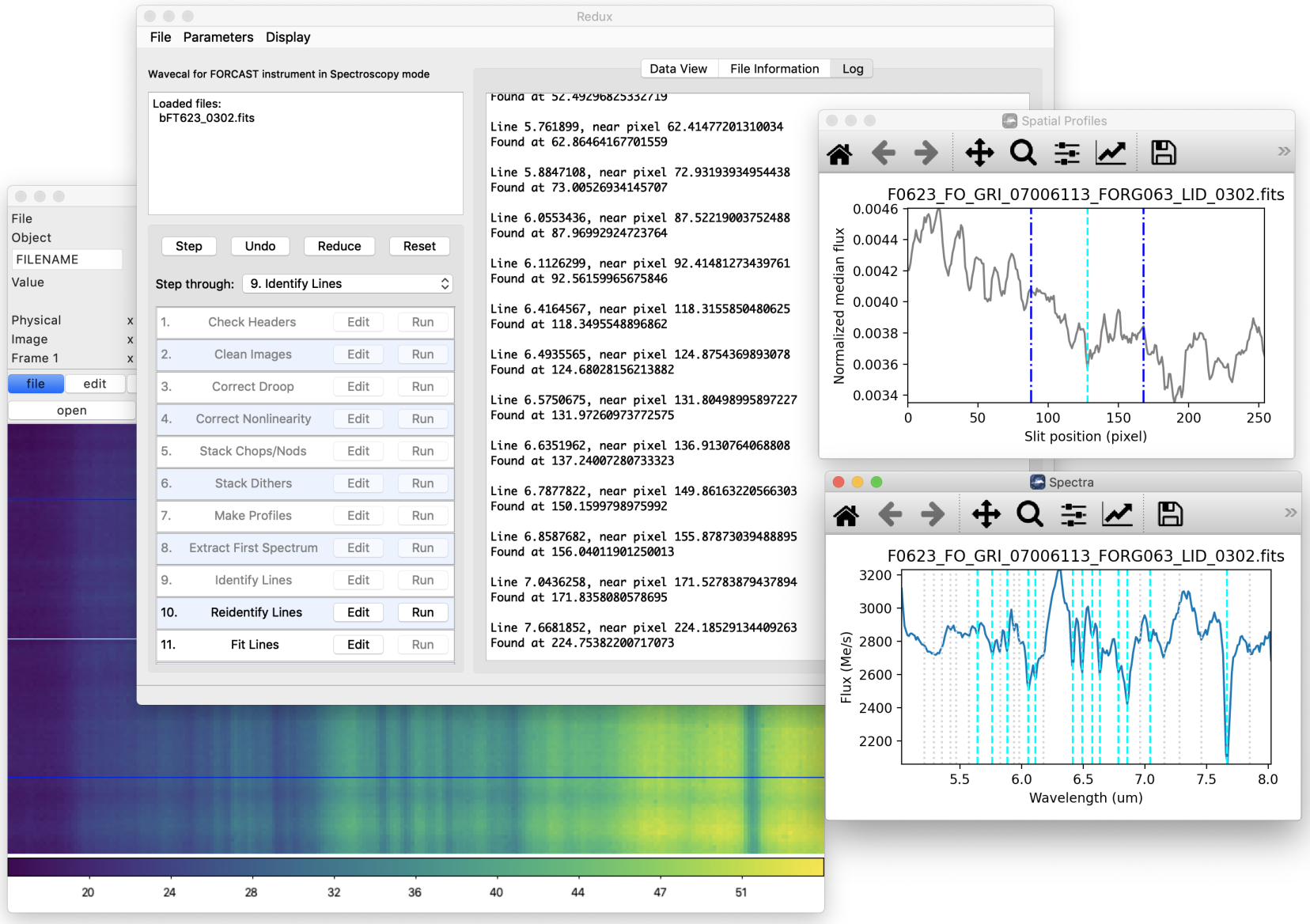
Fig. 96 Wavecal mode reduction and diagnostic plots.

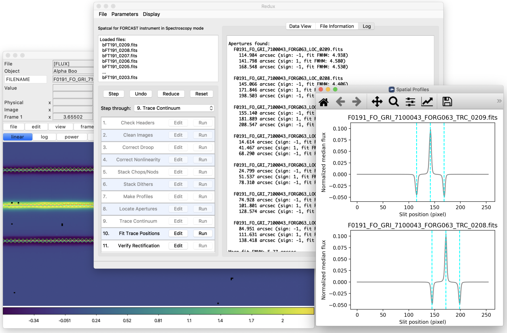
Fig. 97 Spatcal mode reduction and diagnostic plots.

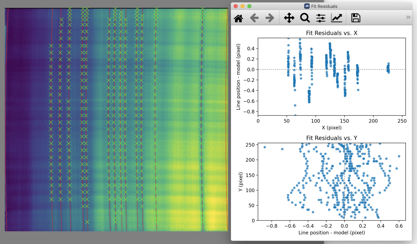
Fig. 98 Wavecal mode fit surface and residuals.

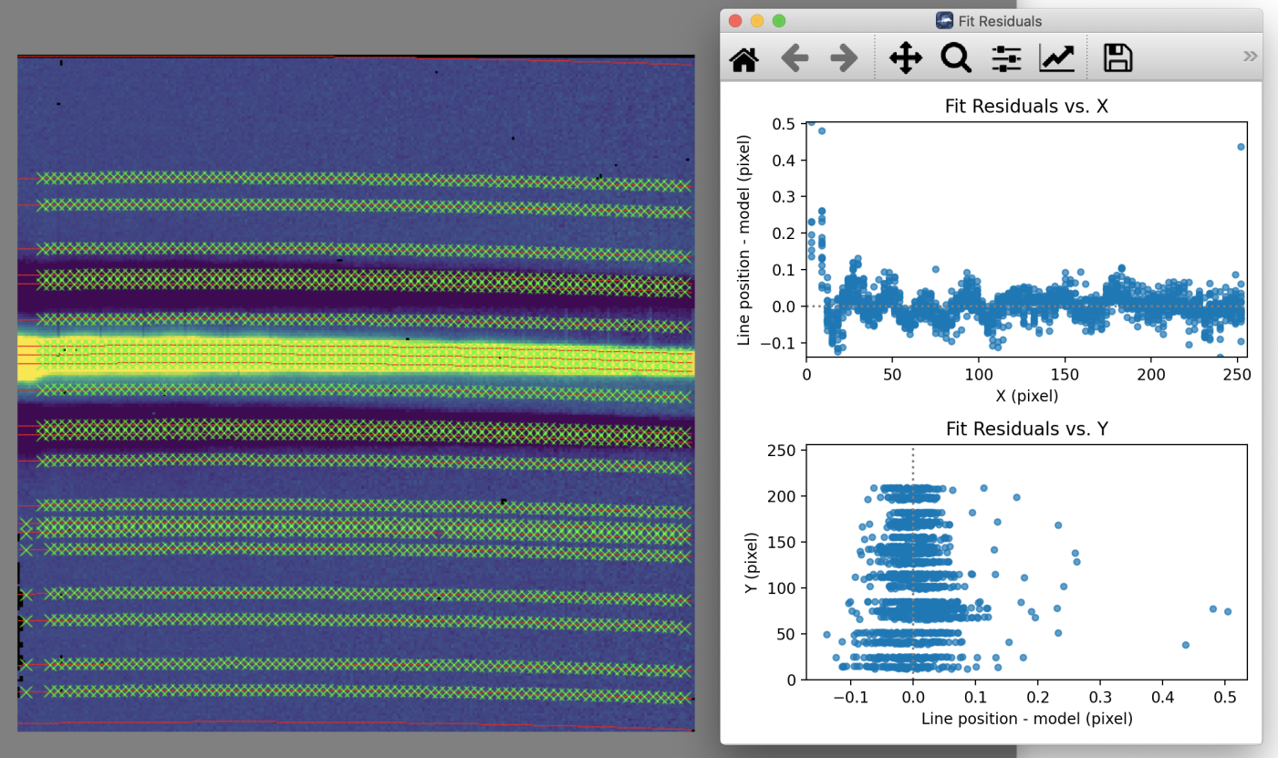
Fig. 99 Spatcal mode fit surface and residuals.

Appendix D: Change notes for the FORCAST pipeline

Significant changes

Below are listed the most significant changes for the FORCAST pipeline over its history, highlighting impacts to science data products. See the data handbooks or user manuals associated with each release for more information.

All pipeline versions prior to v2.0.0 were implemented in IDL; v2.0.0 and later were implemented in Python. An early predecessor to the FORCAST Redux pipeline, called DRIP/FG, was also released for FORCAST reductions in 2013, but no data in the SOFIA archive remains that was processed with this pipeline.

For previously processed data, check the PIPEVERS keyword in the FITS header to determine the pipeline version used.

FORCAST Redux v2.7.0 (2022-12-13)

User manual: Rev. M

Imaging

• Add option to use measured water vapor values from the header (WVZ_OBS) for calibration reference.

Spectroscopy

• Add option to use measured water vapor values from the header (WVZ_OBS) for selecting the atmospheric model used for telluric correction.

FORCAST Redux v2.6.0 (2022-09-12)

User manual: Rev. L

Imaging

• Add options to allow diagnostic reductions in the detector coordinate frame, skipping distortion correction and rotation by the sky angle.

Spectroscopy

• Fix a bug in water vapor optimization, causing the pipeline to return too-low PWV values for observations with strong sky lines and significant wavelength shifts.

FORCAST Redux v2.5.0 (2022-05-25)

User manual: Rev. K

Spectroscopy

• Accommodate slit scan data with asymmetric nods (SKYMODE=SLITSCAN_NXCAC).

FORCAST Redux v2.4.0 (2022-04-06)

User manual: Rev. K

Imaging

• Replace the scikit-image dependency with local implementations of warping and image interpolation algorithms.

Spectroscopy

• Add a line list overplot feature to the spectral viewer for interactive pipeline reductions.

FORCAST Redux v2.3.0 (2021-06-14)

User manual: Rev. J

Spectroscopy

• Improve the automatic wavelength shifting algorithm in the flux calibration step to be more reliable across a larger range of wavelength shifts.

• Additional features for the spectral viewer: reference overplots and enhanced feature fitting options.

FORCAST Redux v2.2.1 (2021-04-14)

User manual: Rev. H

Imaging

• Fix NaN handling in peak-finding algorithm for centroid registration.

• Fix expected units for TGTRA keyword, used for non-sidereal target registration.

FORCAST Redux v2.2.0 (2021-03-10)

User manual: Rev. H

All modes

• Add preview images (*.png files) for all final data products.

Spectroscopy

• In GUI mode, replace static spectral plots with an interactive viewer.

FORCAST Redux v2.1.0 (2020-09-01)

User manual: Rev. G

Imaging

• Add BUNIT keys for all extensions.

• Fix for NaN handling with some image combination methods.

Spectroscopy

• Fix WAVEPOS extension in spectral cube (SCB) to match wavelengths of the cube slices.

• Fix for wavelength shift optimization occasionally reporting spurious shifts.

• Add support for wavelength/spatial calibration file generation to the pipeline. The output product is a WCL file (PRODTYPE=wavecal); it may be used in the Make Profiles step in the pipeline to update or customize the wavelength calibration.

• Add support for combining and smoothing response files generated from standards (RSP files).

• Add support for generating slit correction images to the pipeline. The output product is a SCR file (PRODTYPE=slit_correction). It may be used in the Make Profiles step to correct for slit response.

• Add SPECSYS=TOPOCENT keyword to FITS headers to indicate that wavelengths have not been corrected for barycentric velocity shifts.

FORCAST Redux v2.0.0 (2020-05-07)

User manual: Rev. F

All modes

• Full reimplementation of the IDL pipeline into Python 3.

• Images and spectral cubes now have the option of registering to a non-sidereal target position, rather than to the sidereal WCS.

Imaging

• Data formats change significantly. Imaging products now separate flux, error, and exposure map into separate FITS image extensions, rather than storing them as a 3D cube in the primary extension. Note that the error (standard deviation) is now stored instead of variance.

Spectroscopy

• Data formats change significantly. Images and spectra are stored in the same FITS file, under separate extensions. Final 1D spectra (CMB files, PRODTYPE=combined_spectrum) are still stored in the same format as before; the spectrum corresponds to the SPECTRAL_FLUX extension in the COA (PRODTYPE=coadded_spectrum) file.

FORCAST Redux v1.5.0 (2019-07-24)

User manual: Rev. E

Imaging

• Incorporate new pinhole masks for distortion correction. Allow different masks by date.

FORCAST Redux v1.4.0 (2019-02-21)

User manual: Rev. E

Spectroscopy

• Introduce support for slit-scan observations. The output product is a spatial-spectral cube (file code SCB, PRODTYPE=speccube, PROCSTAT=LEVEL_4).

FORCAST Redux v1.3.2 (2018-09-06)

User manual: Rev. D

All modes

• Fix input manifest handling to not expect the number of files at the top of the list.

FORCAST Redux v1.3.1 (2018-03-08)

User manual: Rev. D

All modes

• Added ASSC-MSN key to track all input MISSN-ID values, for mosaic support. Also added ASSC-OBS keys to track all input OBS_ID values.

Imaging

• Fix for registration error in mosaics with non-empty COADX/Y0 keys.

FORCAST Redux v1.3.0 (2017-04-24)

User manual: Rev. D

Imaging

• Exposure map is now stored in units of seconds, instead of number of exposures.

• Support for multi-field mosaics is introduced. The Level 4 product type is a MOS file (PRODTYPE=mosaic).

• Extra NaN borders are stripped from images after the merge step.

• Default registration method is now WCS comparison, rather than header shifts from dither keywords.

Spectroscopy

• Incorporated process for generating instrumental response curves into the pipeline. The output product is a response file (RSP) for each telluric standard observation. RSP files can be combined together with a separate tool to generate a master response spectrum.

FORCAST Redux v1.2.0 (2017-01-25)

User manual: Rev. C

Imaging

• Flux calibration procedure revised to separate telluric correction from flux calibration. Telluric correction is now performed on a file-by-file basis, for better accuracy, after registration. The REG file is no longer saved by default; it is replaced by a TEL file which is telluric-corrected but not flux calibration. The final calibration factor is still applied at the end of the pipeline, making a single CAL file. The CALFCTR stored in the header is now the calibration factor at the reference altitude and zenith angle; it no longer includes the telluric correction factor. The latter value is stored in the new keyword TELCORR.

Spectroscopy

• Introduced telluric correction optimization, using a library of ATRAN files at various water vapor values, and using the one that best corrects the data. Derived WV values are stored in the FITPWV keyword.

FORCAST Redux v1.1.3 (2016-09-20)

User manual: Rev. B

Imaging

• Rotation in the merge step is now performed around the CRPIX (boresight center) rather than the image center. This fixed small misalignments among images of fields taken at multiple rotation values.

FORCAST Redux v1.1.2 (2016-07-29)

User manual: Rev. B

Imaging

• Fix for flux calibration procedure to distinguish between Barr2 and Barr3 dichroics.

FORCAST Redux v1.1.1 (2016-06-09)

User manual: Rev. B

Imaging

• Fix for bad NaN handling, leaving small artifacts in merged image.

FORCAST Redux v1.1.0 (2016-01-28)

User manual: Rev. B

Imaging

• Flux calibration factors are now applied to data arrays to convert them to physical units (Jy). The calibrated data product has file code CAL (PRODTYPE=calibrated). COA files are no longer designated Level 3, even if their headers contain calibration factors.

• Border-padding around valid imaging data now has NaN value instead of 0.

FORCAST Redux v1.0.8 (2015-10-06)

User manual: Rev. A

Spectroscopy

• Bug fix for plot generation in headless mode.

FORCAST Redux v1.0.7 (2015-09-03)

User manual: Rev. A

All modes

• Handle DETCHAN keyword set to SW/LW instead of 0/1.

Imaging

• Apply average calibration factors to standards, instead of derived value from photometry

FORCAST Redux v1.0.6 (2015-06-26)

User manual: Rev. A

Imaging

• Fix for negative values in variance plane.

• Stop re-doing photometry for standards when applyin calibration factors.

FORCAST Redux v1.0.5 (2015-05-27)

User manual: Rev. A

All modes

• Introduced the TOTINT keyword, to track the total integration time, as it would be requested in SITE, for more direct comparison with proposals.

FORCAST Redux v1.0.4 (2015-05-14)

User manual: Rev. A

All modes

• Total nominal on-source exposure time now tracked in the EXPTIME keyword.

• Introduced the ASSC_AOR key to track all input AOR-IDs for each reduction.

Imaging

• Flux calibration is now integrated into the pipeline, rather than applied after the fact by a separate package. Flux calibration factors are stored in keywords in the Level 3 data files; they are not directly applied to the data.

• Photometry is automatically performed on flux standard observations, with values stored in FITS keywords.

Spectroscopy

• Introduced spatial correction maps for improved rectified images.

• Introduced slit response functions for detector response correction in the spatial direction.

FORCAST Redux v1.0.3 (2015-01-23)

User manual: Rev. A

All modes

• Nonlinearity correction modified for High/Low capacitance distinction.

• Output filename convention updated to include flight number.

• Introduced date-handling for calibration parameters.

Imaging

• Source positions for standards recorded and propagated in SRCPOSX/Y keywords.

Spectroscopy

• Modifications to default spectral extraction parameters to support extended sources.

• Scale spectra before merging to account for slit loss.

• Introduced option to turn off subtraction of median level from spatial profiles, to support extended sources and short slits.

• Introduced telluric correction and flux calibration.

• ITOT and NEXP keywords introduced to track total integration time.

FORCAST Redux v1.0.2 (2014-07-08)

User manual: Rev. A

Spectroscopy

• G2xG1 wavelength calibration update.

FORCAST Redux v1.0.1 (2014-06-17)

User manual: Rev. A

Imaging

• Flux calibration package (pipecal) integration and improvements.

Spectroscopy

• Wavelength calibration updates.

FORCAST Redux v1.0.0 (2013-12-30)

User manual: Rev. -

All modes

• Integrated FORCAST imaging algorithms (DRIP) with Spextool spectral extraction algorithms, in a standard pipeline interface (Redux).