Fitting Curves to Data

A common desire when exploring data is to fit some kind of line to the data, and the Eye of SOFIA obliges. Through keyboard shortcuts, the user can select a range of data and have a simple two component model fit to the selection. The fit is overplotted on the data for a quick check on if the fit worked, while the parameters of the fit are displayed in a separate window, where they can be saved to file.

The fitting methods are found the the Pane class (described in more detail Plotting). The process of fitting data requires interacting with both the data and the GUI. Only the Pane object has easy access to both. Additionally, if the data has been altered in any way from its original values read from the FITS file (such as changing units), then only the Pane object has access to the data with the correct values.

The kinds of curves available to fit to data are shown in Models Available for Curve Fitting. All models include fitting a baseline model to the data (linear model for spectra, plane for an image). The baseline improves the quality of the fit as the curve itself no longer has to account for any background and can focus more the feature of interest.

Table 41 Models Available for Curve Fitting

Data Type	Model	Available
Spectrum	1D Gaussian	Yes
	1D Moffat	No
	Lorentz	No
	Linear	No
Image	2D Gaussian	No
	2D Moffat	No
	Sersic	No
	Planar	No

Selecting Data

The first step to fitting a curve to data is to select the data to be fit. The process is initialized by pressing the “F” key, setting the figure to selection mode. This uses the same methods as the zooming process to reduce the limits of the plot. While in selection mode the Eye will record the data coordinates of any place the user clicks. When two coordinates are recorded the selection mode ends and the x-coordinates of the points are passed to the Pane object for fitting. The y-coordinates of the points are not used. Currently there are no non-interactive methods for selecting the data range.

Method

Once the data range has been selected it is passed to the perform_fit method of the Pane class, where it determines which kind of model to fit to the data, which determines which fitting method gets called. The first step is to select the subsample of data to apply the curve fitting algorithm to. For each order in each dataset loaded in the pane, all x data within the x-axis limits along with the corresponding y data are retrieved. The y-axis limits are not used. Only data points where both the x and y values are not NaN are used for for fitting.

Once the subset is ready it is used to create a rough initial guess for the curve parameters. For example, a Gaussian fit has amplitude, mean, and stddev parameters. The amplitude is initialized to the y value in the middle pixel less the median y value, the mean is initialized to the x value in the middle pixel, and sigma is initialized to \(1/3\) of the width of the x window. Additionally, bounds to the parameters are set to speed up the curve fit. For a Gaussian all paramters are allowed to span the set of real numbers except for the mean, which is restricted to lie within the x window, and the sigma, which is restricted to positive values less than the width of the x window.

With the initial values set the curve models can be initialized. The Eye uses curve models from the astropy.modeling module. All curves fit to data are a composite of the requested curve and a baseline curve. For example, fitting a Gaussian to a spectrum feature would result in fitting a a combined Gaussian1D and Linear1D model.

The actual fitting is done with scipy’s curve_fit function . While astropy.modeling models have built-in fitting routines, they tend to be unreliable. The scipy routines produce more consistently good fits. However if errors are encountered while fitting, the error is logged and the dataset is skipped. If no errors were raised, the fitted curve is then displayed.

Displaying Results

The results of a curve fit are displayed in two ways. First the curve itself is plotted over the data for visual inspection on the quality of fit. Second the parameters of all fits are displayed in a separate window.

Plotting the curve for a 1D fit involves plotting two distinct lines. The first is the fitted curve itself. The second is a vertical line located at the fit’s centroid. Both of these artists are added to the Gallery class as described in Gallery. An example is shown in Spectrum with Fit.

The separate window is controlled by the FittingResults class. The window is a simple QtTable widget that lists the details of all fits performed, as outlined in Curve Fit Parameters Displayed. An example is shown in Results window. If the fitting method is invoked an additional time, the parameters of the new fit are appended to the end of the table. The table can be cleared of all results with the “Clear Table” button. Additionally the table can be written to a CSV file with the “Save Table” button. If one or more rows are selected when the “Save Table” button is pressed only the selected rows will be written to file.

Table 42 Curve Fit Parameters Displayed

Field	Description
filename	Name of FITS file
order	Spectral order curve was fit to
x_field	Data field on x-axis (e.g. “wavepos”)
y_field	Data field on y-axis (e.g. “spectral_flux”)
mean	Centroid of Gaussian1D fit
stddev	Sigma of Gaussian1D fit
amplitude	Peak value of Gaussian1D fit.
baseline	Value of Linear1D fit at “mean”
base_intercept	y-intercept of Linear1D fit
base_slope	Slope of Linear1D fit
lower_limit	Lower limit of x-coordinates of the fitting window
upper_limit	Upper limit of x-coordinates of the fitting window

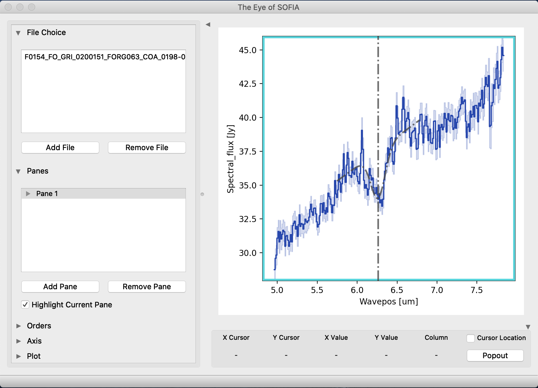
Fig. 134 Eye of SOFIA displaying FORCAST grism data with a Gaussian fit to a feature.

Fig. 135 Parameters for a Gaussian fit to a feature in a FORCAST grism dataset.