Models

Overview

The Model classes are used to store the contents of data sets (FITS files and non-FITS) read into the Eye. The Eye is intended to display any data generated by SOFIA, including grism data, spectral cubes, images, and multi-order spectra. Currently only the spectra viewer is available, so only spectral models are used. Spectral cubes are not yet supported. Currently, all data products from FORCAST and EXES are being supported. We also support data in non-FITS format using General.

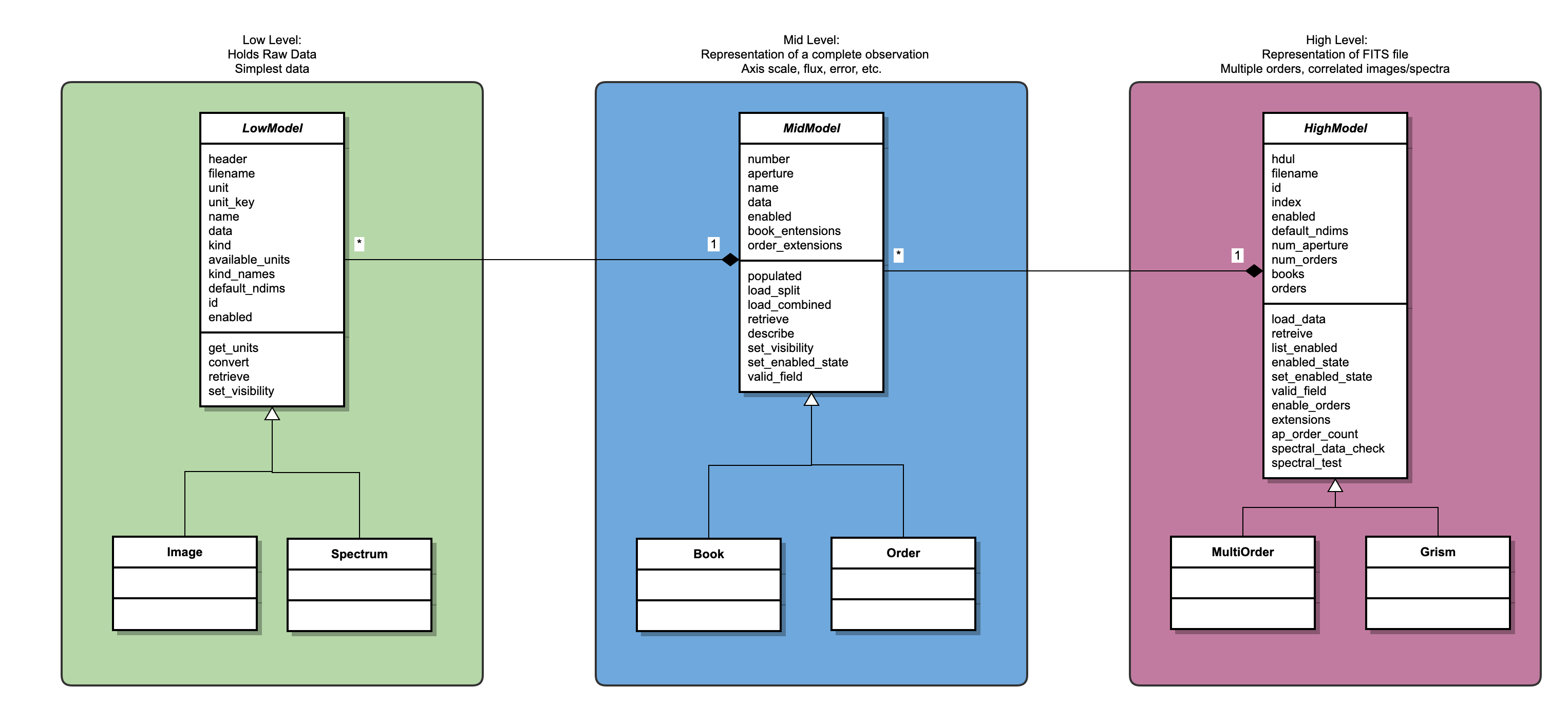
While all data sets are packaged in FITS files, the details of how the data is structured can vary wildly. To simplify the task of plotting, all data sets are read into a collection of Model classes. The method General() converts a non-FITS dataset into HDU format so it can be dealt with in the same manner as a FITS file. There are three levels of Model classes corresponding to more minute details of the data set. The Eye itself only interacts with the top level Model class, which allows for a single uniform interface for the Eye to access any part of the dataset without needing to know the details of how the FITS file was structured.

Diagram

Model Levels

The Model classes are split into three layers:

• High Model: Describes a single FITS file

• Mid Model: Describes a single observation

• Low Model: Describes a single measurement

For example, a calibrated coadded grism file from FORCAST will be loaded into:

• One high model (Grism)

• Two mid models:

  • One for image (Book)

  • One for spectrum (Order)

• Eight low models:

  • FLUX (Image)

  • ERROR (Image)

  • EXPOSURE (Image)

  • WAVEPOS (Spectrum)

  • SPECTRAL_FLUX (Spectrum)

  • SPECTRAL_ERROR (Spectrum)

  • TRANSMISSION (Spectrum)

  • RESPONSE (Spectrum)

Each layer is defined by an abstract class (HighModel, MidModel, and LowModel) that is implemented by a variety of subclasses. The details of each subclass are defined below.

High Models

High models describe a single FITS file. They are uniquely defined by their id, which is the same os their filename. Currently the HighModel abstract class is implemented in two subclasses:

• Grism: The grism describes a FITS file that contains both a single image and a single spectrum. Any data product from FORCAST is read into a Grism class.

• MultiOrder: The multiorder class describes a FITS file that contains multiple spectra and no images. This is primarily used for EXES data products.

Mid Models

Mid models describe a singe observation. This means all the data contained in a mid model are related to each other and describe different aspects a single piece of data. There are two MidModel subclasses:

• Book: For two dimensional datasets (ie images).

• Order: For one dimensional datasets (ie spectra)

Low Models

Low models describe a single measurement, or quantity. Here is where the actual data resides, as well as everything needed to describe the data. This includes the kind of data it is (e.g. flux or time), the data’s units, and the data’s name (e.g. “flux” or “exposure”). There are two LowModel subclasses:

• Image: For a two dimensional data array.

• Spectrum: For a one dimensional data array

Interaction Between Levels

Interactions between the model levels is tightly controlled and abstracted as much as possible. The goal is to have a model system that is as flexible as possible, so adding new datasets to the Eye’s capabilities is as painless as possible. As such each layer knows nothing about the layer above it and very little about the contents of the layer below it. They are largely self-contained. Additionally the interactions are kept generic, so the same function calls work regardless of the nature of the data.

The best example of this philosophy in action is the retrieve method. For example, to plot a spectrum data on an axis, the Pane object needs to get the raw data describing the flux and the wavelengths for a specific order of a specific grism object. Rather than accessing the data directly through a series of complicated chained indexing, each model layer implements a “retrieve” method. Using this, the Pane object requests the raw data (level = “raw”) of the field (“spectral_flux”) from an order (“0”) of the Grism. The Grism find the correct Order and asks for the raw spectral_flux data. The Order finds the Spectrum with the the “spectral_flux” name and asks for its raw data. The Spectrum returns the numpy array containing the raw data back up the chain until the Pane gets. The same process happens for the “wavepos” data and now Pane can plot a spectrum. This seemingly convoluted process exists so the inner relations between the model layers are free to change at any point in the future and only the “retrieve” method will need to be updated. The Pane class has no need to know how the models are structured, only how to ask the Grism for data. This process also allows for proper error checking to ensure only valid data is returned and invalid requests do not crash the Eye.

Reading in Data

Loading High Model

Initializing a HighModel and populating it with data is initialized by the interface contained in the Model class. The interface has only one method add_model, which accepts either a filename or a FITS header data unit list (HDUL). If a filename is given, the file is opened to obtain an HDUL. Based on the instrument name contained the in “INSTRUME” keyword of the header, the correct HighModel subclass is instantiated with the full HDUL following the logic in Selection Rules for HighModel Subclasses.

Table 37 Selection Rules for HighModel Subclasses

Instrument	HighModel
FORCAST	Grism
EXES	MultiOrder

Loading Mid Model

The HDUL is passed to the load_data method of the appropriate HighModel. The next step is simple for a MultiOrder object. A number of Order objects are created equal to the number of orders in the HDUL header keyword “NORDERS”. A Grism object must first determine the correct mixture of Book and Order objects that are required to accurate encapsulate the data (there can be either one or zero of each kind, in any combination). Currently this is decided by examining the file description contained in the file name, as summarized in Selection Rules for Grism Contents. This is not reliable, however, and will be improved in future releases.

Table 38 Selection Rules for Grism Contents

Grism Structure	File Codes
Contains no spectra	APS, BGS, CLN, DRP, LNZ, LOC, STK, TRC
Contains no images	CAL, CMB, IRS, MRG, RSP, SPC
Contains both	COA,

An order is loaded in by passing the HDUL, the filename, and the order’s number to Order. Different data products lay out the spectral data across the HDUL in two different formats: split and combined. For an order to be valid, for each pixel in the spectrum it must contain the corresponding wavelength, the measured flux, and the associated flux error. An order can have the instruments response and the atmospheric transmission for each pixel as well. A split order will have each parameter in a separate extension of the HDUL, while a combined order will have all data in a single extension. The split format is the standard for calibrated FORCAST products, but EXES and earlier FORCAST products will use the combined. The Order initialization determines what format to use based on the dimensions of the HDUl. If the HDUL contains only one extension, then it must be a combined order. Otherwise, it is assumed to be a split order. Since this is based on the total size of the HDUl and not just the spectral parts, it will assume that all grism data sets with an associated image use the split format.

Loading a combined order requires assumptions about how the dataset has been written. All parameters are combined into a single two dimensional numpy array where each row corresponds to a measured parameter and each column corresponds to a pixel in the spectrum. However what parameter is in each row is not contained anywhere in the HDUL, so it must be assumed using the pattern in Layout of Combined Order.

Table 39 Layout of Combined Order

Row	Parameter	Label	Unit Keyword	Kind
1	Wavelength	wavepos	XUNITS	wavelength
2	Flux	spectral_flux	YUNITS	flux
3	Flux Error	spectral_error	YUNITS	flux
4	Total Transmission	transmission	None	scale
5	Instrument Response	response	None	scale

Each row in the HDUL’s data is split off and passed to the Spectrum initializer with the name of the “Label” column and the kind of the “Kind” column. The name used is the same as the extension name for the same parameter in split orders, and the kind is used to define what unit conversions are possible for the data. Not all combined orders have all the parameters listed, so the loading process iterates through the rows available, assuming they all follow this same structure.

Loading a split order is easier as fewer assumptions are made. Each parameter has been assigned its own extension in the HDUL, so to load the order merely requires passing each extension to the Spectrum initializer. The name is the same as the extension’s name so no assumptions are made. There are no assumptions as to the order of the each parameter, either in relation to each other or in the HDUL as a whole, as the entire HDUL is parsed. This means any extensions that actually represent images are also checked here. To prevent attempts to parse an image into a spectrum, the shape of the extension’s data array is checked. Only arrays with one dimension are parsed into a Spectrum object while arrays with two dimensions are passed.

The image version of an Order is the Book class. It follows much of the same structure as the Order` class in that it instantiate a series of Image objects for each parameter contained in the FITS file. The data for each parameter is a two dimensional numpy array. The parameters might be split across several extensions in the HDUL or they might be combined into a single extension whose data is a three dimensional array. In the case of a combined HDUL the data is split off into the corresponding parameters and passed into an individual Image object. This requires assumptions about the structure of the data cube which have not been implemented yet as image viewing is not a feature of the Eye.

Loading Low Model

The low models available are Image and Image. A particular LowModel` instance is unique defined by the HUDL’s filename and a “name” (either pulled from the extension or given by the parent Order). An additional important parameter is “kind”, which describes what type of data the model will hold. If the “kind” is not passed in when the LowModel is initialized then it is determined from the “name”, following the pattern in Available Kinds of Low Models.

Table 40 Available Kinds of Low Models

Low Model	Kind	Matching Names
Image	scale	transmission
	position	aperture_trace
	unitless	badmask
		spatial_map
	flux	flux
		error
		spectral_flux
		spectral_error
	time	exposure
Spectrum	scale	transmission
		response
		response_error
	unitless	spatial_profile
	flux	spectral_flux
		spectral_error
	wavelength	wavepos
		slitpos
	position	slitpos

The “kind” is important as it determines what units are valid for each LowModel, as well as determining if a dataset can be added to a plot with exiting data on it (only matching kinds can be plotted against each other without utilizing overplots). Aside from the different available “kind”s and the data shape, the Spectrum and Image classes are very similar.

In addition to characterizing the type of data, low models oversee unit conversions. The actual conversion is done in by making calls to the unit_conversion module, but the low models configure the calls. The unit_conversion module utilizes the astropy.units package to handle the details the actual conversion.