Basic Usage Example

import numpy as np
from sofia_redux.toolkit.resampling import Resample, resample

x = np.arange(10)
y = x + 100

# initialize the Resample object
resampler = Resample(x, y)
y2 = resampler(4.5)  # get the resampled result at x = 4.5

# or perform the resampling in a single step with resample
y2 = resample(x, y, 4.5)

Fitting noisy data

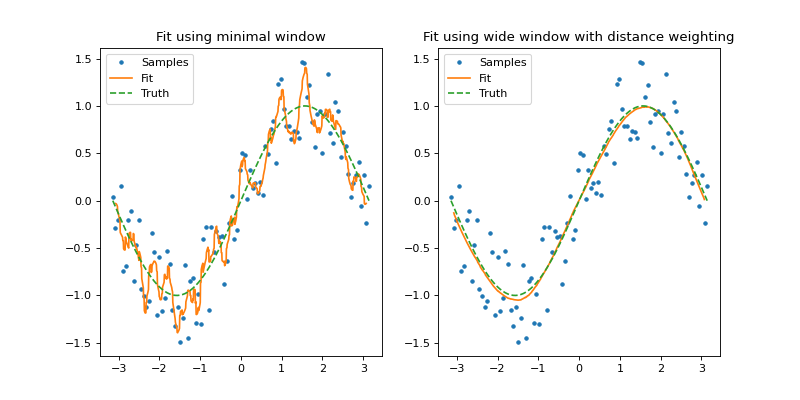
In the following example we generate two second order polynomial fits to a noisy sine wave. In the first plot (left), we use a minimal window (default) sufficient to allow for at least 3 (order + 1) samples per resampling point. This produces a rather jagged plot that represents the data on a small local scale. Please note that this is only recommended when we know the sample spacing is regular since the default window is taken from stochastic analysis of the sample distribution.

In the second plot, a fit is generated using a much wider window (\(\pi / 2 \approx 25 \text{ samples}\)) and a distance weighting parameter of 0.4 (\(\alpha = 0.4\)) which is more representative of the true sine function.

import numpy as np
import matplotlib.pyplot as plt
from sofia_redux.toolkit.resampling import Resample

rand = np.random.RandomState(100)
noise = rand.rand(100) - 0.5
x = np.linspace(-np.pi, np.pi, 100)
ytrue = np.sin(x)
y = ytrue + noise
xout = np.linspace(-np.pi, np.pi, 1000)

narrow_resampler = Resample(x, y, order=2)
yfit = narrow_resampler(xout)
plt.figure(figsize=(10, 5))
plt.subplot(121)
plt.plot(x, y, '.', label='Samples')
plt.plot(xout, yfit, label='Fit')
plt.plot(x, ytrue, '--', label='Truth')
plt.legend()
plt.title("Fit using minimal window")

wide_resampler = Resample(x, y, window=np.pi / 2, order=2)
yfit2 = wide_resampler(xout, smoothing=0.4, relative_smooth=True)
plt.subplot(122)
plt.plot(x, y, '.', label='Samples')
plt.plot(xout, yfit2, label='Fit')
plt.plot(x, ytrue, '--', label='Truth')
plt.legend()
plt.title("Fit using wide window with distance weighting")

(Source code, png, hires.png, pdf)

Multiple data-sets

If you wish to perform resampling multiple times from a fixed set of input coordinates to a fixed set of output coordinates with different data, error, or mask values then it is preferable to do this with a single Resample object than creating multiple instances. In this case, all data should be supplied on initialization.

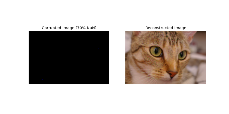
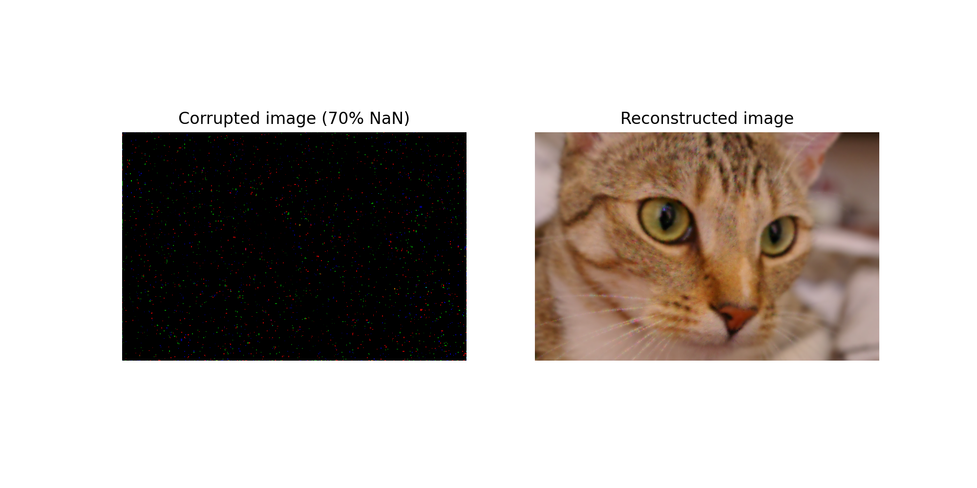
The following example does this to correct a corrupted RGB image, where each R-G-B slice represents a different data set that shares input and output coordinate mappings with all other sets.

from sofia_redux.toolkit.resampling import Resample
import imageio
import numpy as np

image = imageio.imread('imageio:chelsea.png').astype(float)
s = image.shape
rand = np.random.RandomState(42)
bad_pix = rand.rand(*s) < 0.7  # 70 percent corruption
bad_image = image.copy()
bad_image[bad_pix] = np.nan

y, x = np.mgrid[:s[0], :s[1]]
coordinates = np.vstack([c.ravel() for c in [x, y]])

yout = np.arange(s[0])
xout = np.arange(s[1])

# supply data in the form (nsets, ndata)
data = np.empty((s[2], s[0] * s[1]), dtype=float)
for frame in range(s[2]):
    data[frame] = bad_image[:, :, frame].ravel()

resampler = Resample(coordinates, data, window=10, order=2)
good = resampler(xout, yout, smoothing=0.1, relative_smooth=True,
                 order_algorithm='extrapolate', jobs=-1)

# get it b1ack into the correct shape and RGB format for plotting
good = np.clip(np.moveaxis(good, 0, -1).astype(int), 0, 255)

# Use the original good pixel coordinates where available
good[~bad_pix] = bad_image[~bad_pix]

plt.figure(figsize=(10, 5))
plt.subplot(1,2,1)
plt.axis('off')
plt.imshow(bad_image / 255)
plt.title("Corrupted image (70% NaN)")

plt.subplot(1,2,2)
plt.axis('off')
plt.imshow(good)
plt.title("Reconstructed image")

(Source code, png, hires.png, pdf)

Order limits and edge clipping

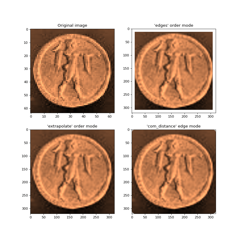
The following example uses a 3rd order polynomial to resample an image (top-left) onto a finer resolution grid. The top-right image was generated using the default edge mode 'com_distance' (see order mode) which only permits resampling if enough samples bound a resampling point in both the x and y directions. This is the safest option but does result a NaN border. The bottom-left image uses order_algorithm='extrapolate' to permit resampling regardless of the sample distribution so long as enough unique samples exist to perform fitting. Finally, the bottom-right image uses the “com_distance” edge mode (see edge clipping) to only perform fits if the samples are within a certain threshold from the coordinate center-of-mass of samples within the window.

Note that an optimal window selection is performed by the resampler since the samples (pixels in this case) are regularly spaced and the window parameter was omitted during initialization. A small smoothing parameter has been used to preserve detail.

from sofia_redux.toolkit.resampling import Resample
import imageio
import numpy as np

image = imageio.imread('imageio:coins.png')
image = image / image.max()
image = image[12:76, 303:367]  # 64 x 64 pixel image

y, x = np.mgrid[:image.shape[0], :image.shape[1]]
coordinates = np.vstack([c.ravel() for c in [x, y]])

# default resampler
resampler = Resample(coordinates, image.ravel(), order=3)

# blow up by a factor of 5
xout = np.linspace(0, 63, 64 * 5)
yout = np.linspace(0, 63, 64 * 5)

# Default uses "bounded" order algorithm
bounded_mode = resampler(xout, yout, smoothing=0.05,
                         relative_smooth=True, order_algorithm='bounded',
                         jobs=-1)
extrap_mode = resampler(xout, yout, smoothing=0.05,
                        relative_smooth=True,
                        order_algorithm='extrapolate', jobs=-1)
com_edges = resampler(xout, yout, smoothing=0.05,
                      order_algorithm='extrapolate',
                      edge_threshold=0.8, relative_smooth=True, jobs=-1)

plt.figure(figsize=(10, 10))
plt.subplot(221)
plt.title("Original image")
plt.imshow(image, cmap='copper')
plt.subplot(222)
plt.imshow(bounded_mode, cmap='copper')
plt.title("'edges' order mode")
plt.subplot(223)
plt.imshow(extrap_mode, cmap='copper')
plt.title("'extrapolate' order mode")
plt.subplot(224)
plt.imshow(com_edges, cmap='copper')
plt.title("'com_distance' edge mode")

(Source code, png, hires.png, pdf)

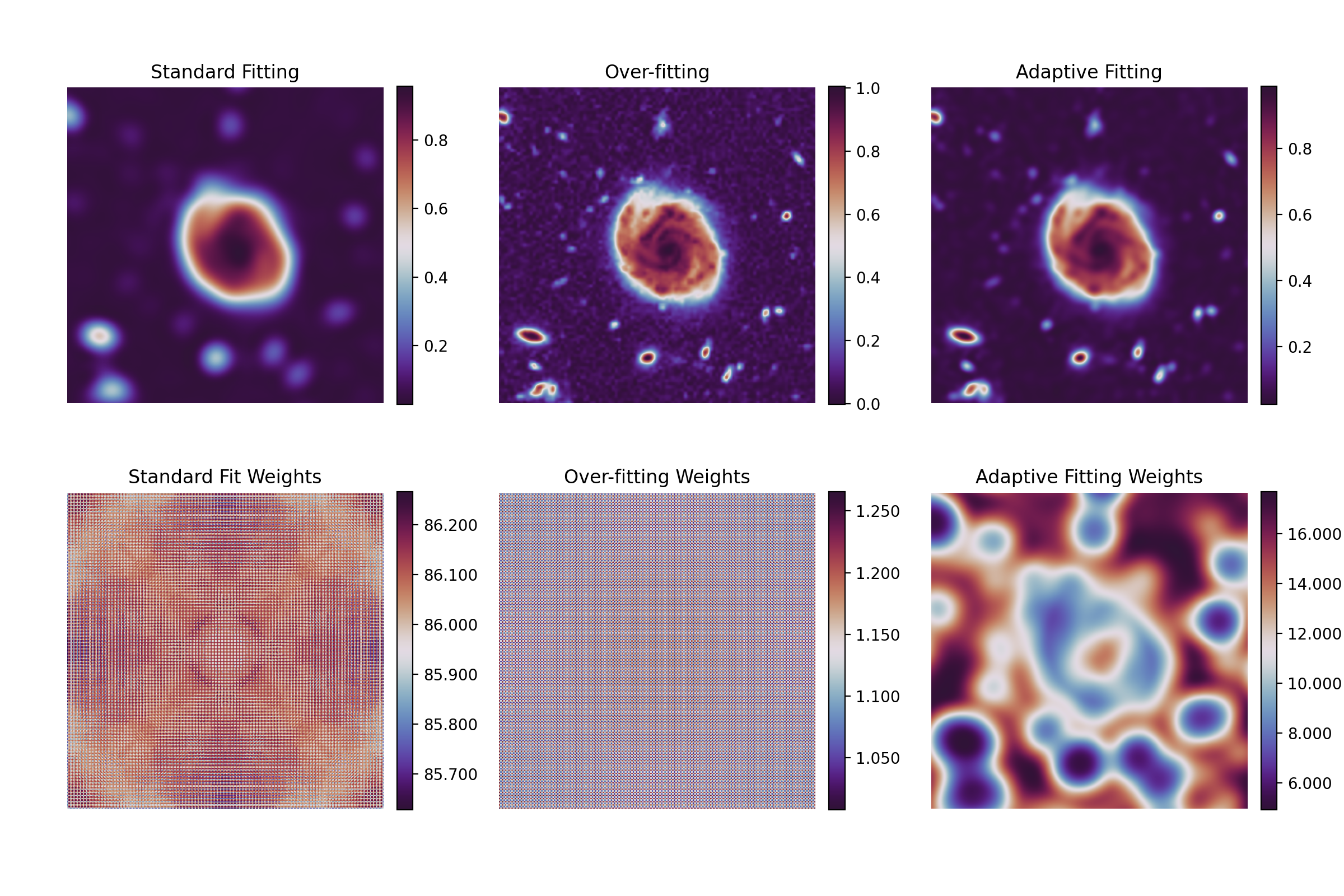
Adaptive Weighting

Please see adaptive_weighting for details on the adaptive weighting algorithm.

The following images and associated weighting maps are generated using the same second order polynomial resampler from a coarse input image (not displayed). The output images are at 3 times the original resolution. A naive approximation to the error and spatial scale was used. The original image was originally had data values in the range [0, 255] scaled into the range [0, 1]. The error was taken to be equal to 1 in the original image which is \(\approx\) 0.003 in the scaled image.

Likewise, the spatial scale was taken to be 3 pixels (each dimension) by eye. It is suggested to use a window region of \(\approx\) 3 times this value when using adaptive weighting. Therefore, the window in each dimension is 9 pixels. Since this is a regular grid of samples, the adaptive_threshold parameter (limit to the minimum contraction of the window) has been set to \(\frac{1}{3}\) so there are always at least 3 samples to fit in both dimensions for a second order polynomial (requires order + 1).

from sofia_redux.toolkit.resampling import Resample
from astropy.stats import gaussian_fwhm_to_sigma
import imageio
import matplotlib.pyplot as plt
import numpy as np

# Cut out a section of the image for analysis
image = imageio.imread('imageio:hubble_deep_field.png')
image = image[325:475, 45:195].sum(axis=-1).astype(float)
image -= image.min()
image /= image.max()
y, x = np.mgrid[:image.shape[0], :image.shape[1]]
coordinates = np.vstack([c.ravel() for c in [x, y]])

# blow up center of the image leaving a border to avoid edge effects
xout = np.linspace(25, 125, 300)
yout = np.linspace(25, 125, 300)

resampler = Resample(coordinates, image.ravel(), order=2, window=9,
                     error=1e-3)

sigma = gaussian_fwhm_to_sigma * 3

low, low_weights = resampler(xout, yout,
                             smoothing=3 * sigma,
                             get_distance_weights=True,
                             order_algorithm='extrapolate', jobs=-1)

high, high_weights = resampler(xout, yout, smoothing=sigma / 3,
                               get_distance_weights=True,
                               order_algorithm='extrapolate', jobs=-1)

adaptive, adaptive_weights = resampler(xout, yout,
                                       smoothing=sigma,
                                       adaptive_threshold=1,
                                       get_distance_weights=True,
                                       order_algorithm='extrapolate',
                                       jobs=-1)

fig, axs = plt.subplots(2, 3, figsize=(12, 8))
for ax in axs.ravel():
    ax.axis('off')
fig.subplots_adjust(left=0.05, right=0.95,
                    wspace=0.25, hspace=0.01,
                    top=0.95, bottom=0.05)
color = 'twilight_shifted'

low_img = axs[0, 0].imshow(low, cmap=color)
axs[0, 0].title.set_text("Standard Fitting")
fig.colorbar(low_img, ax=axs[0, 0], fraction=0.046, pad=0.04)

high_img = axs[0, 1].imshow(high, cmap=color)
axs[0, 1].title.set_text("Over-fitting")
fig.colorbar(high_img, ax=axs[0, 1], fraction=0.046, pad=0.04)

adapt_img = axs[0, 2].imshow(adaptive, cmap=color)
axs[0, 2].title.set_text("Adaptive Fitting")
fig.colorbar(adapt_img, ax=axs[0, 2], fraction=0.046, pad=0.04)

wlow_img = axs[1, 0].imshow(low_weights, cmap=color)
axs[1, 0].title.set_text("Standard Fit Weights")
fig.colorbar(wlow_img, ax=axs[1, 0], fraction=0.046, pad=0.04,
             format='%.3f')

whigh_img = axs[1, 1].imshow(high_weights, cmap=color)
axs[1, 1].title.set_text("Over-fitting Weights")
fig.colorbar(whigh_img, ax=axs[1, 1], fraction=0.046, pad=0.04,
             format='%.3f')

wadapt_img = axs[1, 2].imshow(adaptive_weights, cmap=color)
axs[1, 2].title.set_text("Adaptive Fitting Weights")
fig.colorbar(wadapt_img, ax=axs[1, 2], fraction=0.046, pad=0.04,
             format='%.3f')

(Source code, png, hires.png, pdf)

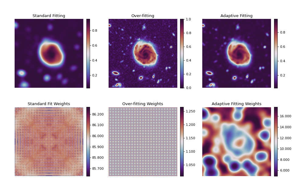
The left-most images display the result and associated weight map using these parameters without adaptive weighting. Note however, that smoothing=1/3 conveys a different meaning depending on whether adaptive weighting is enabled or not (see enabling_adaptive for details). The middle image and weight map were generated using a very fine resolution weighting parameter of 0.01 resulting in something very close to the original image. Here, pixel-to-pixel noise variation can clearly be seen.

Finally, the right-most image and weight map were created using the adaptive weighting algorithm. Pixel-to-pixel noise variation can no longer be seen while details are preserved. Examining the adaptive weight map generally shows which areas are smoother (high weight) and which areas preserve more of the details (low weight).